

Excel allows us to lookup values in two ways. Using the VLOOKUP function or with INDEX and MATCH functions. The MATCH function returns a row for a value in a table, while the INDEX returns a value for that row. This step by step tutorial will assist all levels of Excel users in learning the different ways of lookups.
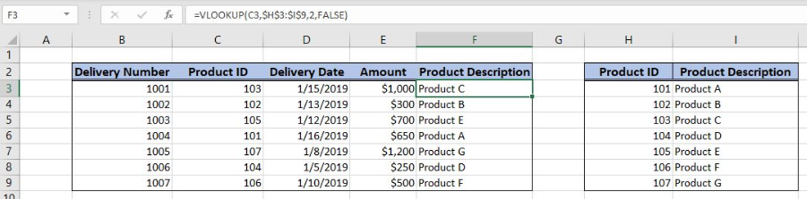 Figure 1. The final result of the formula
Syntax of the VLOOKUP formula
The generic formula for the VLOOKUP function is:
=VLOOKUP(lookup_value, table_array, col_index_num, range_lookup)
The parameters of the VLOOKUP function are:
- lookup_value – a value that we want to find in a table_array
- table_array – a range in which we want to lookup
- col_index_num – a column number in table_array from which we would like to get a value
- range_lookup – default value is FALSE. This means that we want to find an exact match for a lookup value.
Syntax of the INDEX formula
The generic formula for the INDEX function is:
=INDEX(array, row_num, column_num)
The parameters of the INDEX function are:
- array – a range of cells where we want to get a data
- row_num – a number of a row in the array for which we want to get a value
- column_num – a column in the array which returns a value.
Syntax of the MATCH formula
The generic formula for the MATCH function is:
=MATCH(lookup_value, lookup_array, [match_type])
The parameters of the MATCH function are:
- lookup_value – a value which we want to find in the lookup_array
- lookup_array – the array where we want to find a value
- [match_type] – a type of match. We put 0 which is an exact match.
Setting up Our Data for the Examples
Our table consists of 5 columns: “Delivery Number” (column B), “Product ID” (column C), “Delivery Date” (column D), “Amount” (column E) and “Product Description” (column F).
In column F, we want to populate a Product Description from the Lookup table in the range H3:I9. This table consists of 2 columns: “Product ID” (column H) and “Product Description” (column I). Two tables are joined by the columns “Product ID”.
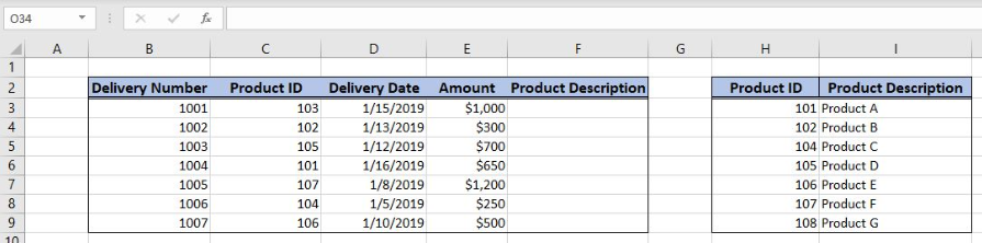 Figure 2. Data that we will use in the example
Using the VLOOKUP Formula
In the first example, we will use the VLOOKUP function. We want to get a product description in the cell F3, from the lookup table H3:I9, based on the Product ID 103 in the cell C3.
The formula looks like:
=VLOOKUP(C3, $H$3:$I$9, 2, FALSE)
The lookup_value parameter is C3. The table_array is $H$3:$I$9. The range must be fixed, as it’s not changing when the formula is copied to the other cells. The col_index_num is 2 because we want to get a value from the second column. The range_lookup is FALSE.
To apply the VLOOKUP formula, we need to follow these steps:
- Select cell F3 and click on it
- Insert the formula:
=VLOOKUP(C3, $H$3:$I$9, 2, FALSE) - Press enter
- Drag the formula down to the other cells in the column by clicking and dragging the little “+” icon at the bottom-right of the cell.
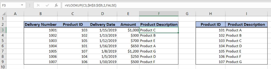 Figure 3. Using the VLOOKUP formula
The function returns “Product C” in F3 as this is the description for the Product ID 103 from C3.
Using the INDEX and MATCH Formula
Now, we will do the same example using the INDEX and MATCH functions.
The formula looks like:
=INDEX($H$3:$I$9, MATCH(C3, $H$3:$H$9, 0), 2)
The lookup_value parameter of the MATCH function is C3. The lookup_array is $H$3:$H$9, while the match_type is 0, as we want the exact match. The result of the MATCH function is the row_num parameter of the INDEX function. The array the range $H$3:$I$9.
To apply the formula, we need to follow these steps:
- Select cell F3 and click on it
- Insert the formula:
=INDEX($H$3:$I$9, MATCH(C3, $H$3:$H$9, 0), 2) - Press enter
- Drag the formula down to the other cells in the column by clicking and dragging the little “+” icon at the bottom-right of the cell.
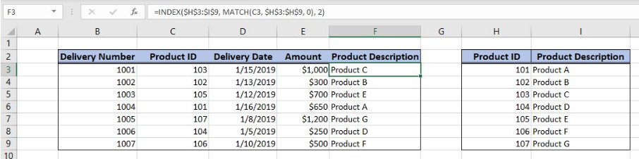 Figure 4. Using the INDEX and MATCH Formula
Again, the result in the cell F3 is the same as in the previous example with VLOOKUP – “Product C”.
Most of the time, the problem you will need to solve will be more complex than a simple application of a formula or function. If you want to save hours of research and frustration, try our live Excelchat service! Our Excel Experts are available 24/7 to answer any Excel question you may have. We guarantee a connection within 30 seconds and a customized solution within 20 minutes.


Leave a Comment