

The EXACT function works as a lookup tool. However, it is case-sensitive. This function compares two text strings and returns TRUE if they are exactly the same, FALSE otherwise. In this post, EXACT will be used with SUMPRODUCT function to illustrate how EXACT function works.
Exact match lookup with SUMPRODUCT
Generic Formula
=SUMPRODUCT(--(EXACT( value , lookup_array)), amount_array)
Although SUMPRODUCT works with arrays, it does not require using array shortcut (CTRL + SHIFT + ENTER). You can complete a SUMPRODUCT formula by simply pressing ENTER after typing the formula.
Example
Considering the example below, the formula in D5 is:
=SUMPRODUCT(--(EXACT(E4,B2:B8)),C2:C8)
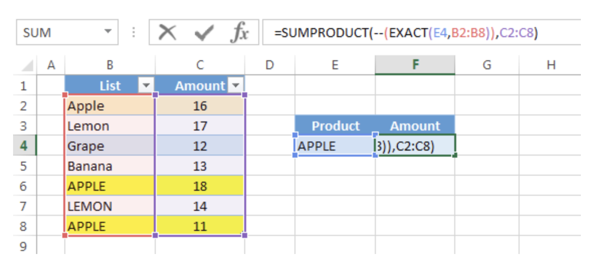
Figure 1 – Exact match lookup with SUMPRODUCT
In this case, standard lookups like VLOOKUP of HLOOKUP will ignore case and return the first match, which is “Apple”. However, the EXACT function will match the exact cases in the lookup_array. The result will be 29:
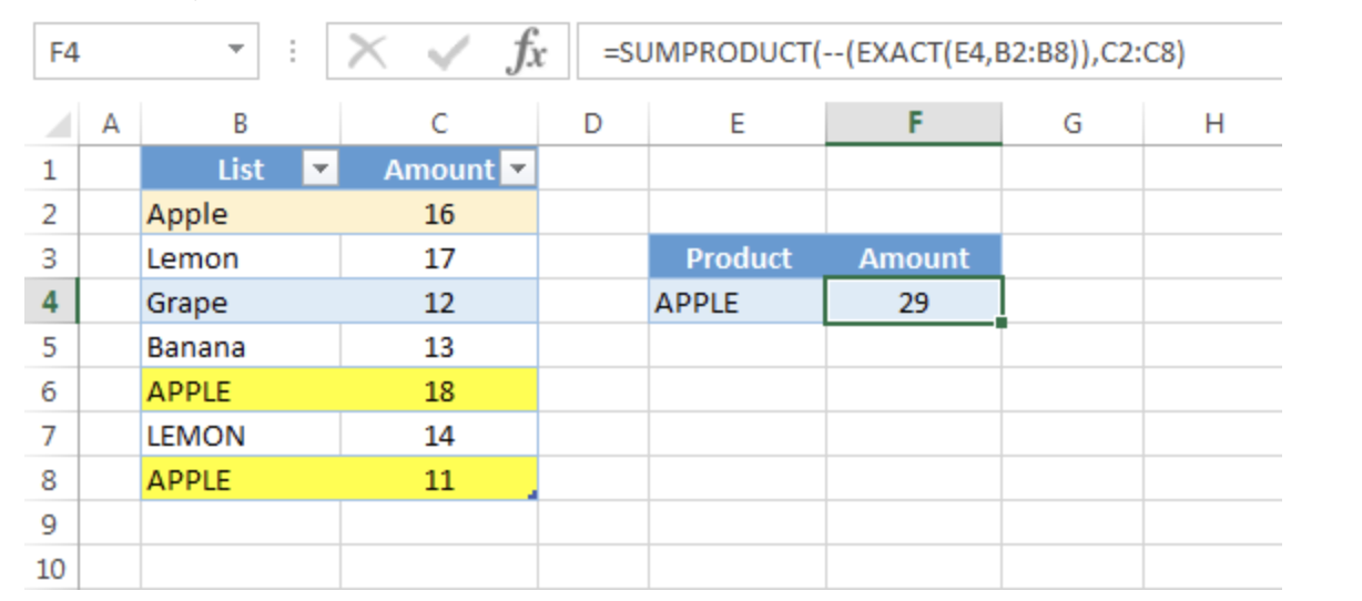
Figure 2– Exact match lookup with SUMPRODUCT
Explanation of formula
How this formula works:
EXACT(E4,B2:B8)
: this portion produces an array like this
{FALSE; FALSE; FALSE; FALSE;TRUE; FALSE;TRUE}
– The double unary operator (–) is used to convert the array to 1 and 0. A new array is returned like this: {0;0;0;0;1;0;1}
You can also produce 1 and 0 arrays in this way: EXACT(E4,B2:B8)*1
– SUMPRODUCT then simply multiples the items in two array: {0;0;0;0;1;0;1} and {16;17;12;13;18;14;11}. The returned array is: {0;0;0;0;18;0;11}. Finally, it sums all the values and returns 28.
Note:
- This formula will only work with numeric values. SUMPRODUCT doesn’t retrieve text.
- All arrays in SUMPRODUCT formula must have the same number of rows and columns otherwise you will get the #VALUE! error
Still need some help with Excel formatting or have other questions about Excel? Connect with a live Excel expert here for some 1 on 1 help. Your first session is always free.


Leave a Comment