

While working with Excel, we are able to determine the row number of any cell or reference by using the ROW function. This step by step tutorial will assist all levels of Excel users in the usage and syntax of the ROW function.
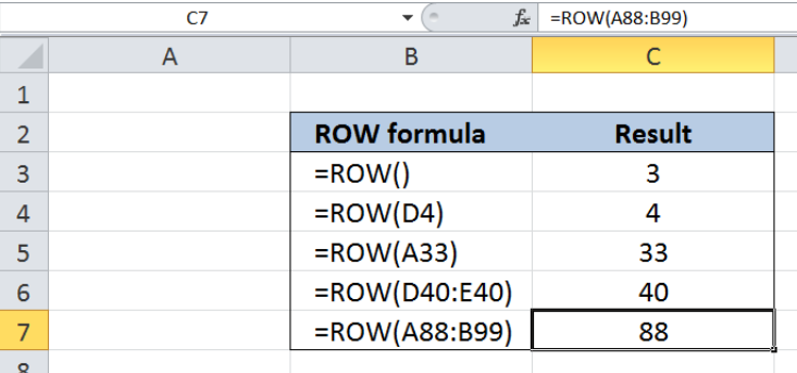 Figure 1. Final result: Excel ROW function
Syntax of the ROW function
ROW function returns the row number of a reference
=ROW(reference)
- reference – The cell or range of cells whose row number we want to determine
- When reference is not given, ROW function returns the row number of the cell containing the formula
Setting up our Data
Our data consists of two columns: ROW formula (column B) and Result (column C). We want to enter the ROW formulas in column B and see the results in column C.
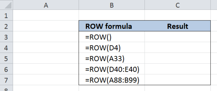 Figure 2. Sample data to determine the row number
Determine the row number of a certain cell
In order to determine the row number of a certain cell containing the ROW function, we leave the reference argument blank. Let us follow these steps:
Step 1. Select cell C3
Step 2. Enter the formula: =ROW()
Step 3. Press ENTER
As a result, the value in cell C3 is 3, because cell C3 is in the third row of the worksheet.
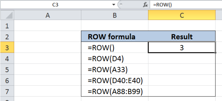 Figure 3. Using ROW function to determine the row number of a certain cell
Determine the row number of any cell
In order to determine the row number of any cell in the worksheet, we use the ROW function and enter the cell reference as the argument. We want to know the row number of cell D4. Let us follow these steps:
Step 1. Select cell C4
Step 2. Enter the formula: =ROW(D4)
Step 3. Press ENTER
As a result, the value in C4 is 4, because cell D4 is in the fourth row of the worksheet. ROW function returns only the row number, regardless of the column number of the cell.
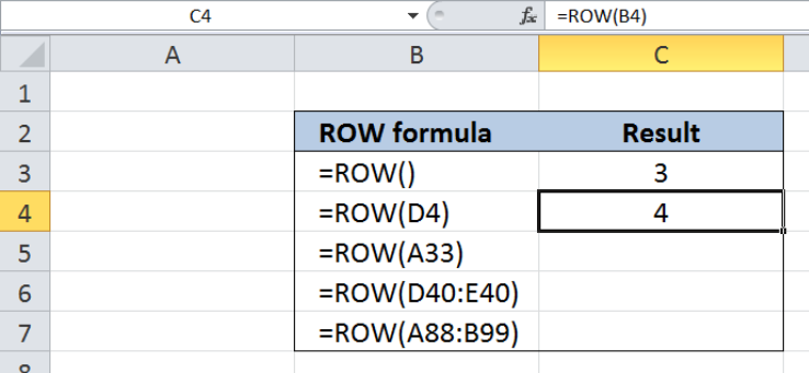 Figure 4. Using ROW function to determine the row number of D4
In a similar manner, entering the formula =ROW(A33) in cell C5 will result to the value “33”, because A33 is located in the 33rd row of the worksheet.
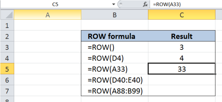 Figure 5. Using ROW function to determine the row number of A33
Determine the row number with range as reference
When a range is used as a reference argument in the ROW function, the value returned is the row number of the upper leftmost cell in the range. Let us follow these steps:
Step 1. Select cell C6
Step 2. Enter the formula: =ROW(D40:E40)
Step 3. Select cell C7
Step 4. Enter the formula: =ROW(A88:B99)
Step 5. Press ENTER
As a result, the value in cell C6 is 40, because cell D40 is the upper leftmost cell in the range D40:E40 and its row number is 40. In cell C7, the resulting value is 88, because A88 is the upper leftmost cell in the range A88:B99 and its row number is 88.
Below table shows the results in cells C3:C7, where the row number of the given cells is returned by the ROW function.
 Figure 6. Output: Row number with range as reference argument
Instant Connection to an Expert through our Excelchat Service
Most of the time, the problem you will need to solve will be more complex than a simple application of a formula or function. If you want to save hours of research and frustration, try our live Excelchat service! Our Excel Experts are available 24/7 to answer any Excel question you may have. We guarantee a connection within 30 seconds and a customized solution within 20 minutes.


Leave a Comment