

The Excel LOOKUP function returns a value from a range of cells (one column or one row) or an array (multiple rows and columns) based on the approximate match as per the Vector or Array syntax. In this article, we will learn how to use the LOOKUP function with the Vector and Array syntax.
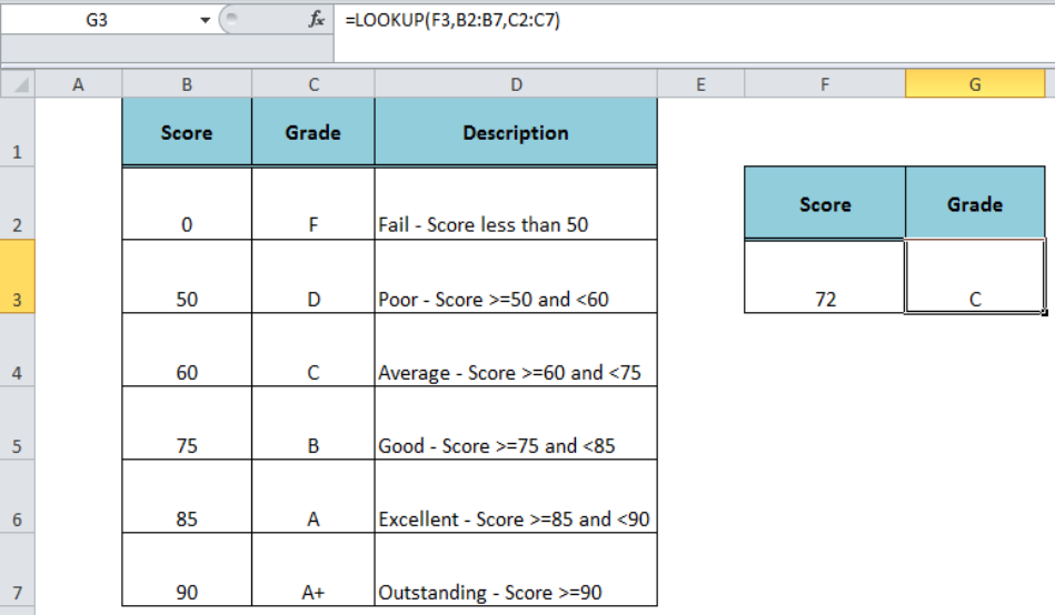 Figure 1. How to Use Excel LOOKUP Function
Syntax For The LOOKUP Function
The LOOKUP Function has the following two forms of syntax;
- Vector Syntax – This syntax is used to look up the value in one column or one row and it returns the value from the corresponding position in the specified column or a row.
- Array Syntax – This syntax is used to look up the value in an array consisting of multiple columns and rows.
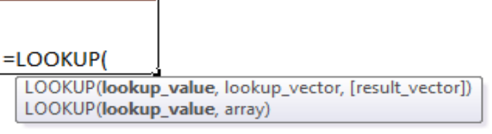 Figure 2. The Syntax Forms Of The LOOKUP Function
Vector Syntax
The vector syntax form of the Lookup function is as follows;
=LOOKUP(lookup_value, lookup_vector, result_vector)
Where,
- Lookup_value – It is a value that needs to be matched
- Lookup_vector – It is the range of one column or row
- Result_vector – It is the optional range of one column or one row from which we need to return the value. If this argument is omitted the function returns the matching value from the lookup_vector range.
Suppose we have listed a score structure in range B2: B7 (lookup_vector) and the relative grades in range C2: C7 (result_vector). We need to return the grade from the result_vector range, based on the approximate match of the given score in the lookup_vector, such as;
=LOOKUP(F3,B2:B7,C2:C7)
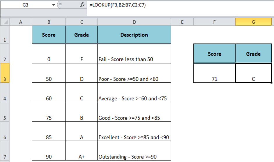 Figure 3. The Vector Syntax For the LOOKUP Function
Array Syntax
The array syntax form of the Lookup function is as follows;
=LOOKUP(lookup_value, array)
The lookup_value is searched based on the following array dimensions:
- If the array contains more columns than rows, then function searches in the first row.
- If rows are more than or equal to columns, then function searches in the first column.
- The function returns the value from the same position in the last corresponding row or column
In our example, we need to use the following formula as per the array syntax to return the grades for the given score;
=LOOKUP(F3, B2: C7)
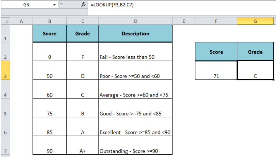 Figure 4. The Array Syntax For the LOOKUP Function
Instant Connection to an Expert through our Excelchat Service:
Most of the time, the problem you will need to solve will be more complex than a simple application of a formula or function. If you want to save hours of research and frustration, try our live Excelchat service! Our Excel Experts are available 24/7 to answer any Excel question you may have. We guarantee a connection within 30 seconds and a customized solution within 20 minutes.


Leave a Comment