Excel CHOOSE Function

Selecting a value from any list can be done by using the CHOOSE function  This step by step tutorial will assist all levels of Excel users in the usage and syntax of the CHOOSE function.  

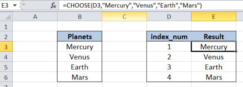Figure 1.  Final result:  Excel CHOOSE function

Formula 1: =CHOOSE(D3,"Mercury","Venus","Earth","Mars")

Formula 2: =CHOOSE($D3,B$3,B$4,B$5,B$6)

Syntax of CHOOSE Function

CHOOSE function returns a value from a list of values based on the index number provided

=CHOOSE(index_num, value1, [value2], ...)

• index_num  – the index number determines which value in the list is returned by the CHOOSE function
  • Index_num must be a number between 1 and 254, or a cell reference with values between 1 and 254
  • Value1 is returned if index_num is 1, values2 if index_num is 2; and so on
  • CHOOSE returns the error #VALUE! if index_num is less than 1 or greater than the number of the last value in the list
• value1, value2, …   the values in the list  that the function chooses from; Only value 1 is required, succeeding values are optional

Setting up our Data

Here we have a list of Planets in column B, and index_num in column D with values from 1 to 4.  We want to choose a value from the list using the index number in column D. The results will be recorded in column E.  

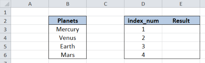Figure 2.  Sample data in using CHOOSE function

Selecting a value from the list using CHOOSE

In order to choose a value from our list of planets using the CHOOSE function, let us follow these steps:

Step 1.  Select cell E3

Step 2.  Enter the formula: =CHOOSE(D3,"Mercury","Venus","Earth","Mars")

Step 3.  Press ENTER

Step 4:  Copy the formula in cell E3 to cells E4:C6 by clicking the “+” icon at the bottom-right corner of cell E3 and dragging it down

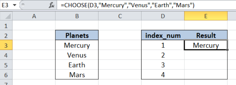Figure 3.  CHOOSE returning the first value in the list

CHOOSE finds a value in the list based on the given index number.  In cell E3, the index number provided is D3, or the value 1. Hence, our formula returns the first value in the list which is “Mercury”.  

In the succeeding cells E4, E5 and E6, our CHOOSE function returns the second, third and fourth value in the list, respectively.  The resulting values are shown below.

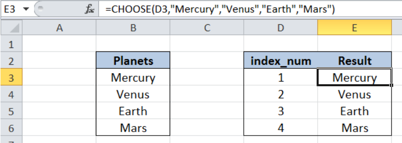Figure 4.  CHOOSE returning values in the list corresponding to index_num

CHOOSE function using cell reference

While using CHOOSE function, we can also use cell references to represent the values in our list.  Let us follow these steps:

Step 1.  Select cell E3

Step 2.  Enter the formula: =CHOOSE($D3,B$3,B$4,B$5,B$6)

Step 3.  Press ENTER

Step 4:  Copy the formula in cell E3 to cells E4:C6 by clicking the “+” icon at the bottom-right corner of cell E3 and dragging it down

The procedure is still the same as in the previous example.  Note that we have used cell references here, instead of hardcoding the values in the list within our formula.  The table below shows the same results for the CHOOSE function in column E.

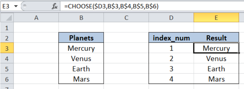Figure 5. CHOOSE returning the same values by using cell references

Most of the time, the problem you will need to solve will be more complex than a simple application of a formula or function. If you want to save hours of research and frustration, try our live Excelchat service! Our Excel Experts are available 24/7 to answer any Excel question you may have. We guarantee a connection within 30 seconds and a customized solution within 20 minutes.