

While working with Excel, we are able to find exact matches that satisfy certain criteria by using the IF, INDEX and MATCH functions. This step by step tutorial will assist all levels of Excel users in extracting data with the aid of a helper column.
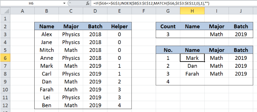 Figure 1. Final result: Extract data with helper column
Formula for Name: =IF($G6<=$G$3,INDEX($B$3:$E$12,MATCH($G6,$E$3:$E$12,0),1),"")
Formula for Major: =IF($G6<=$G$3,INDEX($B$3:$E$12,MATCH($G6,$E$3:$E$12,0),2),"")
Formula for Batch: =IF($G6<=$G$3,INDEX($B$3:$E$12,MATCH($G6,$E$3:$E$12,0),3),"")
Syntax of the IF function
IF function evaluates a given logical test and returns a TRUE or a FALSE
=IF(logical_test, [value_if_true], [value_if_false])
- The arguments “value_if_true” and “value_if_false” are optional. If left blank, the function will return TRUE if the logical test is met, and FALSE if otherwise.
Syntax of the INDEX function
INDEX function returns a value from within a range, as specified by the row and column number
=INDEX(array, row_num, column_num)
The parameters are:
- array – a range of cells where we want to retrieve some data
- row_num – the row in the array from which we want to retrieve data
- column_num – the column in the array from which we want to retrieve data; if the array has only one column, column_num can be omitted
Syntax of the MATCH function
MATCH function returns the position of a value in a range
=MATCH(lookup_value, lookup_array, [match_type])
The parameters are:
- lookup_value – a value which we want to find in the lookup_array
- lookup_array – the range of cells containing the value we want to match
- [match_type] – optional; the type of match; if omitted, the default value is 1; We use 0 to find an exact match
Syntax of the ROWS function
ROWS function returns the number of rows in a data set
=ROW(array)
- array– an array, range or reference for which we want to determine the number of rows
Setting up Our Data
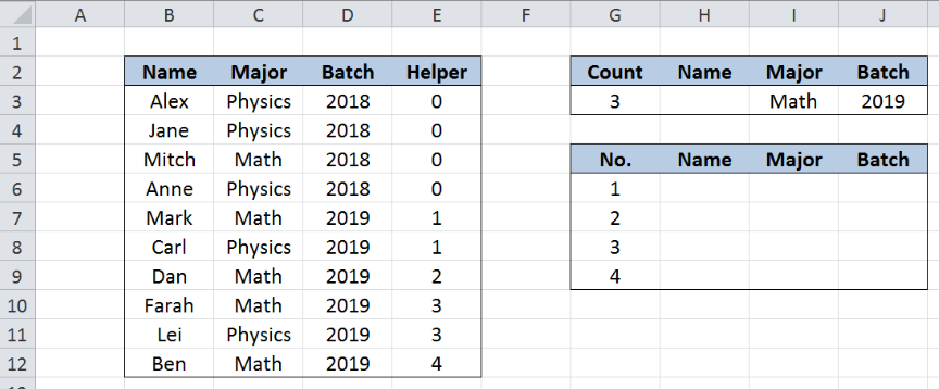 Figure 2. Sample data to extract data with helper column
Our table consists of four columns: Name (column B), Major (column C), Batch (column D) and Helper (column E). Cells G3, I3 and J3 contain our criteria, in this case, count “3”, “Math” for Major and “2019” for Batch. Therefore, we want to find the first three names of Math majors who belong to batch 2019.
Results will be recorded in column H, from H6 down to appropriate number of cells.
Helper Column E
Column E is a helper column that we set-up to aid us in our calculations. In column E, we use the formula:
=SUM(E2,AND(C3=$I$3,D3=$J$3))
to mark the rows matching our criteria.
 Figure 3. Helper column formula
The helper column formula evaluates each row if the values in columns C and D match the criteria “Math” and “2019”, respectively. The two values must match in order for the AND function to return TRUE. A TRUE result has a value 1, while FALSE returns a zero “0” value.
Hence, for every row that matches the two criteria, the helper column formula generates a count, and the value remains the same until it finds the next match. As shown above, the first count “1” is in E7, while the next count “2” is in E9. In row 8 where the criteria are not met, the count in E8 remains at 1, which is the same value as the cell above it.
Extract first three names with “Math” and “2019”
We want to identify the first three names in the list that match the criteria “Math” and “2019” with the help of our helper column (column E). Let us follow these steps:
Step 1. Select cell H6
Step 2. Enter the formula: =IF($G6<=$G$3,INDEX($B$3:$E$12,MATCH($G6,$E$3:$E$12,0),1),"")
Step 3: Press ENTER
Step 4: Copy the formula in cell H6 to cells H7:H9 by clicking the “+” icon at the bottom-right corner of cell H6 and dragging it down
The dollar signs “$” in the formula fix the cells so that we can easily copy and paste the formula to other cells.
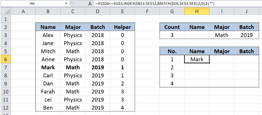 Figure 4. Using INDEX, MATCH and ROWS to find the first match
Our INDEX formula looks up the name of the first match, using the MATCH function to determine the row number. The array for the INDEX function is the range B3:E12, while the column number is 1, because the names are in the first column, B.
Our lookup_value for the MATCH function is G6 or 1. MATCH looks for the value “1” in our helper column with values {0;0;0;0;1;1;2;3;3;4}. The value 1 is the fifth value in the array so the MATCH function returns 5. MATCH function only considers the first match.
Finally, the INDEX function returns the fifth row in the range B3:B12, which is B7, or Mark”. The result displayed in cell H6 is “Mark”, who is the first name who matches the criteria.
For the second and third names, our formula returns the names “Dan” and “Farah” in cells H7 and H8, respectively.
Note that we have a fourth match, Ben in row 12. This is where the IF function comes in. The count that we entered in our criteria in G3 is only “3”, so the IF function ensures that our formula only returns the first three names and cell H9 is left blank.
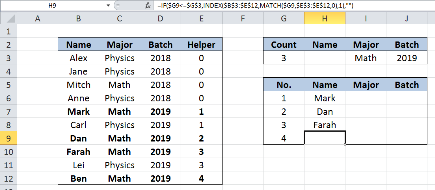 Figure 5. Output: Extract first three names that match “Math” and “2019”
Note:
In order to return the corresponding values for “Major” and “Batch” for each name, we can follow the same procedure but we change the column number for our INDEX formula.
For “Major”, enter the formula with column number 2:
=IF($G6<=$G$3,INDEX($B$3:$E$12,MATCH($G6,$E$3:$E$12,0),2),"")
For “Batch”, enter the formula with column number 3:
=IF($G6<=$G$3,INDEX($B$3:$E$12,MATCH($G6,$E$3:$E$12,0),3),"")
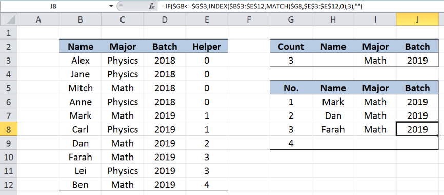 Figure 6. Output: Extract data for Major and Batch
Most of the time, the problem you will need to solve will be more complex than a simple application of a formula or function. If you want to save hours of research and frustration, try our live Excelchat service! Our Excel Experts are available 24/7 to answer any Excel question you may have. We guarantee a connection within 30 seconds and a customized solution within 20 minutes.


Leave a Comment