How to Use the Excel IFNA Function

We can use the excel IFNA function to generate a custom result when a formula ought to display the #N/A error. This function doesn’t detect other errors apart from the #N/A error. The steps below will walk through the process.

Figure 1: How to Use the Excel IFNA Function

Formula

=IFNA(VLOOKUP(D4,A4:B10,2,FALSE),"Not applicable")

Setting up the Data

• We will set up the data by inputting the SUBJECTS for a student in Column A
• Column B contains the scores for each subject
• Column E is where we want the formula to return the result. We will use a VLOOKUP formula to check for the scores of the subjects if they are in the range (A4:B10)

Figure 2: Setting up the Data

Excel IFNA Function

• We will click on Cell E4
• We will insert the formula below into the cell
• =IFNA(VLOOKUP(D4,A4:B10,2,FALSE),"Not applicable")
• We will press the enter key

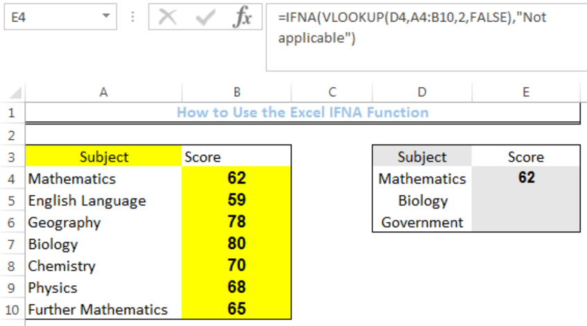Figure 3: Result of VLOOKUP for Cell E4

• We will click on Cell E4 again
• We will double-click on the fill handle (the small plus sign at the bottom right of Cell E4) and drag down to copy the formula into the other cells

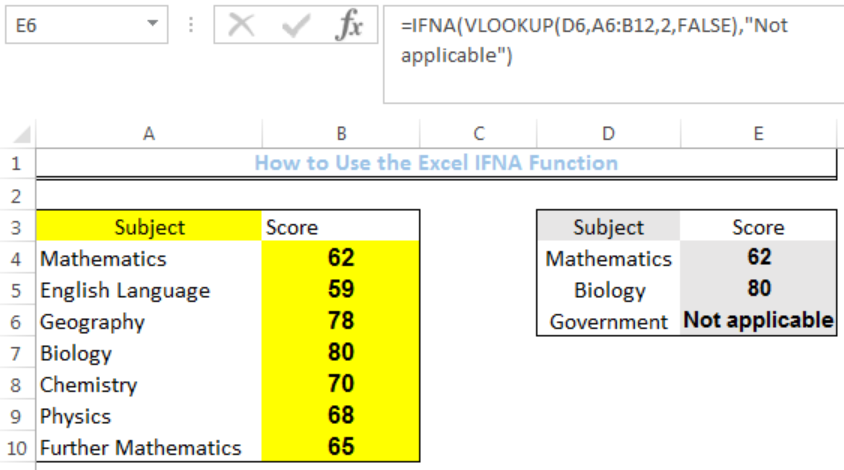Figure 4: Result of Using the IFNA function

Without the IFNA Function

Without the IFNA Function, the formula for VLOOKUP is: =VLOOKUP(D4,A4:B10,2,FALSE). If we clear the data from Cell E4 to Cell E6 where our result is and input the formula below, our result will be like figure 5.

Formula: =VLOOKUP(D4,A4:B10,2,FALSE)

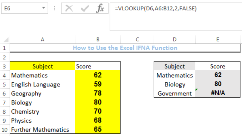Figure 5: Without the IFNA Function

Instant Connection to an Expert through our Excelchat Service

Most of the time, the problem you will need to solve will be more complex than a simple application of a formula or function. If you want to save hours of research and frustration, try our live Excelchat service! Our Excel Experts are available 24/7 to answer any Excel question you may have. We guarantee a connection within 30 seconds and a customized solution within 20 minutes.