

Excel allows a user to use a multiple nested logical expression in order to check if conditions are true. This is possible by using the nested IF function which returns Boolean TRUE or FALSE as a result. This step by step tutorial will assist all levels of Excel users in using the nested IF function.
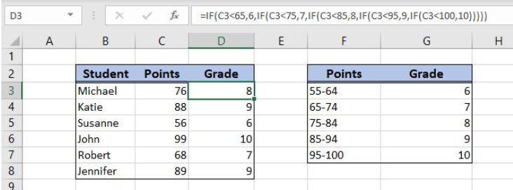 Figure 1. The result of the nested IF function
Syntax of the IF Formula
The generic formula for the IF function is:
=IF(logical_test, value_if_true, value_if_false)
The parameters of the IF function are:
- logical_test – a logical expression that we want to check
- value_if_true – a value which the function returns if a logical_test is TRUE
- value_if_false – a value which the function returns if a logical_test is FALSE.
Setting up Our Data for the Nested IF Function
The first table consists of 3 columns: “Student” (column B), “Ponts” (column C) and “Grade” (column D). The second table is the grade scale and has 2 columns: “Points” (column F) and “Grade” (column G). Based on a number of the points, we want to get a grade for each student in column D, using the points scale in the second table.
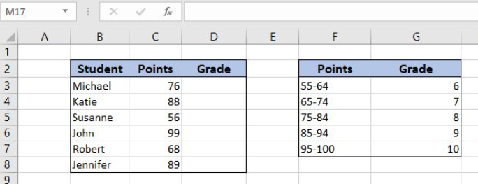 Figure 2. The tables for the nested IF function example
Get a Grade Based on Points Using the Nested IF Function
In our example, to get a grade in the cell D3 for Michael, who has 76 points. In order to do this, we need to check the second table with several nested IF functions.
The formula looks like:
=IF(C3<65,6, IF(C3<75,7, IF(C3<85,8, IF(C3<95,9, IF(C3<100,10)))))
The parameter logical_test for the first IF is C3<65, The value_if_true is the grade 6.If it’s false we need to check further in the next points scale. Therefore, the value_if_false is IF(C3<75,7, IF(C3<85,8, IF(C3<95,9, IF(C3<100,10)))). In this way, we check for every points scale, until 100 points.
To apply the nested IF function, we need to follow these steps:
- Select cell D3 and click on it
- Insert the formula:
=IF(C3<65,6, IF(C3<75,7, IF(C3<85,8, IF(C3<95,9, IF(C3<100,10))))) - Press enter
- Drag the formula down to the other cells in the column by clicking and dragging the little “+” icon at the bottom-right of the cell.
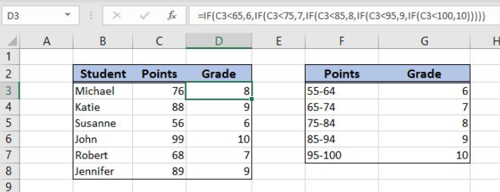 Figure 3. Using the nested IF function to get a grade for the number of points
First, we check if C3 (76 points) is less than 65. As this is not true, we go to value_if_false and check the next IF. Here we check if C3 is less than 75. Again, this is not true, so we are going to value_if_false and entering the third IF function. Now, we check if C3 is less than 85. This is true, so the grade in D3 is 8 (value_if_true of the third IF function).
Most of the time, the problem you will need to solve will be more complex than a simple application of a formula or function. If you want to save hours of research and frustration, try our live Excelchat service! Our Excel Experts are available 24/7 to answer any Excel question you may have. We guarantee a connection within 30 seconds and a customized solution within 20 minutes.


Leave a Comment