Group arbitrary text values

While working with Excel, one of the easiest ways to retrieve data from another table is by using the VLOOKUP function. This step by step tutorial will assist all levels of Excel users in grouping arbitrary text values with the help of the VLOOKUP function.  

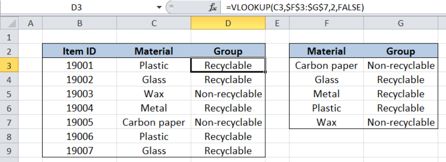Figure 1. Final result: Group arbitrary text values

Final formula:  =VLOOKUP(C3,$F$3:$G$7,2,FALSE)

Syntax of the VLOOKUP function

VLOOKUP is used when we want to look up a value and retrieve data from a given data set.

=VLOOKUP(lookup_value, table_array, col_index_num, [range_lookup])

The parameters of the VLOOKUP function are:

• lookup_value – the value that we want to search and find in the table_array
• table_array – the range of cells in the source table containing the data we want to retrieve
• col_index_num – the column number in the table_array corresponding to the information we want to retrieve, relative to the lookup_value
• [range_lookup] – optional; value is either TRUE or FALSE
  • if TRUE or omitted, VLOOKUP returns either an exact or approximate match
  • if FALSE, VLOOKUP will only find an exact match

Setting up Our Data

Our table contains a list of Item ID (column B) and Material (column C). In column D, we want to   group the materials, whether recyclable or non-recyclable, based on the values in table F2:G7. Cells F2:G7 contain the list of Material (column F) and the corresponding Group per material (column G).

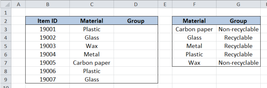Figure 2. Sample data to group arbitrary text values

Group the items using VLOOKUP

We want to group the items according to their material, based on the list in table F2:G7.  In order to populate column D with the values from table F2:G7 using VLOOKUP, we follow these steps:

Step 1.  Select cell D3

Step 2.  Enter the formula: =VLOOKUP(C3,$F$3:$G$7,2,FALSE)

Step 3:  Press ENTER

Step 4:  Copy the formula in cell D3 to cells D4:D9 by clicking the “+” icon at the bottom-right corner of cell D3 and dragging it down

The dollar signs “$” in the formula fix the cells so that we can easily copy and paste the formula to other cells.  

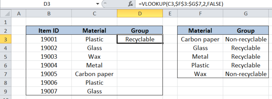Figure 3. Entering the formula to group materials using VLOOKUP

Our lookup_value is cell C3 which is the material.  The table_array is the range F2:G7, where we want to lookup the group per material.  “Group” is in the second column of the table_array so col_index_num is 2.  Range_lookup is FALSE because we want to find the exact match.  

The final result in cell D3 is Recyclable, which is the group where the material “Plastic” belongs.  

Copying the formula to the succeeding cells finally groups all the items according to their material, whether “Recyclable” or Non-recyclable”.  

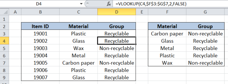Figure 4. Output: Group items according to their material

Note:  When VLOOKUP doesn’t find a match to our lookup value, the function returns the value #N/A.

Most of the time, the problem you will need to solve will be more complex than a simple application of a formula or function. If you want to save hours of research and frustration, try our live Excelchat service! Our Excel Experts are available 24/7 to answer any Excel question you may have. We guarantee a connection within 30 seconds and a customized solution within 20 minutes.