

Excel and Google sheets provide us with several options to freeze cells so they don’t disappear in the screen when we scroll through our data. This step by step tutorial will assist all levels of Excel users to freeze rows and columns in Excel, Google sheets and Mac.
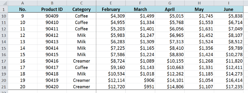 Figure 1. Final result: How to freeze cells in Excel
How to freeze cells in Excel
The Freeze Panes toolbar under View tab in Excel offers three options:
- Freeze Panes
- Freeze Top Row
- Freeze First Column
 Figure 2. Excel Freeze Panes drop-down menu
Suppose we have a large set of data and we want to freeze rows and columns in the following manner:
- Freeze top row only
- Freeze multiple rows
- Freeze first column only
- Freeze multiple columns
- Freeze multiple rows and columns
How to freeze or lock top row in Excel
Freezing only the top row is rather easy. We can click anywhere on our data and follow these steps:
Step 1. Click the View tab
Step 2. Click the Freeze Panes button
Step 3. Select the “Freeze Top Row” option
 Figure 3. Excel Freeze top row
When we scroll down our data, notice that the top row (row 1) is locked such that it is always displayed on screen.
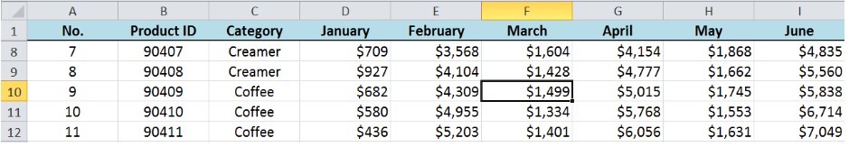 Figure 4. Output: How to lock top row in Excel
How to unfreeze cells in Excel
In order to unfreeze locked cells in Excel, we only need to click View tab > Freeze Panes > Unfreeze Panes.
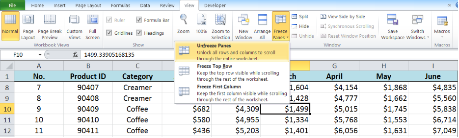 Figure 5. Excel Unfreeze Panes
The cells will automatically unlock and go back to their unfrozen or unlocked state.
 Figure 6. Output: Unfreeze panes in Excel
How to freeze multiple rows in Excel
Suppose we want to lock rows 1 to 6 on the list. To lock multiple rows in Excel, we follow these steps:
Step 1. Select row 7, which is one row after the last row we want to freeze or lock.
Step 2. Click the View tab > Freeze Panes button
Step 3. Select the “Freeze Panes” option
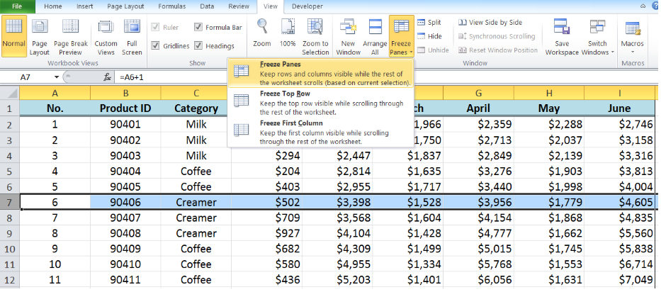 Figure 7. Click Excel Freeze Panes to freeze multiple rows
Note that when we scroll down, rows 1 to 6 are locked and are always displayed on the screen.
 Figure 8. Output: How to freeze multiple rows in Excel
However, when we scroll to the right, the first column (column A) is not displayed on the screen. Since only the rows are locked, the columns still tend to disappear when we scroll to the right of our data.
 Figure 9. Columns disappear when only rows are locked
How to freeze first column in Excel
In order to freeze only the first column, we can click anywhere on our data and follow these steps:
Step 1. Click the View tab
Step 2. Click the Freeze Panes button
Step 3. Select the “Freeze First Column” option
 Figure 10. Excel Freeze First Column
When we scroll to the right of our data, the first column is locked such that it is always displayed on the screen.
 Figure 11. First column remains locked when scrolling to the right
How to freeze multiple columns in Excel
Suppose we want to lock columns A to C on the list. To freeze columns in Excel, we follow these steps:
Step 1. Select column D, which is one column to the right of the last column we want to freeze or lock.
Step 2. Click the View tab > Freeze Panes button
Step 3. Select the “Freeze Panes” option
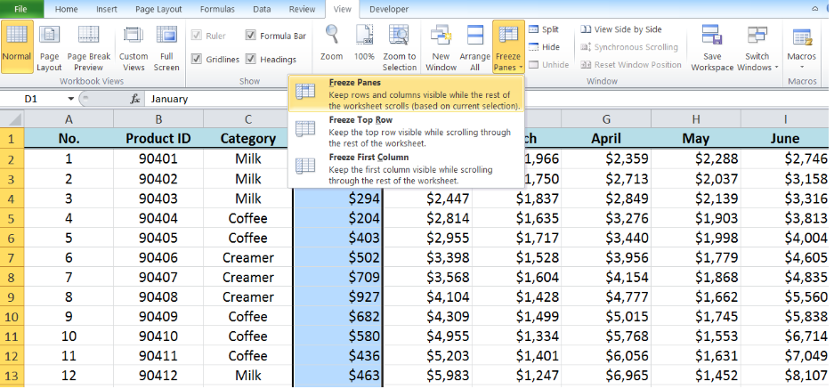 Figure 12. Click Excel Freeze Panes to freeze multiple columns
Now when we scroll to the right, columns A to C are locked and are always visible on the screen.
 Figure 13. Output: How to freeze multiple columns in Excel
However, when we scroll down, the first few rows including the headers are not displayed on the screen. Since only the columns are locked, the rows still tend to disappear when we scroll down our data.
 Figure 14. Rows disappear when only columns are locked
How to freeze multiple cells in Excel
Excel allows us to freeze rows and columns at the same time. This is especially helpful when we are handling a large set of data and there are key cells that we want to be always visible on the screen.
Suppose we want to freeze row 1 and columns A to C on the list so that when we scroll through our data, the headers and important details are always displayed.
In order to freeze multiple rows and columns in Excel, we follow these steps:
Step 1. Select cell D2, which is one row after row 1 and one column after column C
Step 2. Click the View tab > Freeze Panes button
Step 3. Select the “Freeze Panes” option
 Figure 15. Click Excel Freeze Panes to freeze multiple rows and columns
When we scroll down or to the right, the headers in row 1 and the details in columns A to C will always be visible on the screen. Freezing cells are very helpful in analyzing and scanning through large chunks of data.
 Figure 16. Final output: How to freeze cells in Excel
Note:
When freezing multiple rows and columns, we must select the cell which is one row below and one column to the right of the cells we want to freeze.
The rows and columns we want to freeze must be visible in the screen before we press the “Freeze Panes” button. Else, those cells will not be displayed on the screen after the freeze.
Example:
In the image below, cell D2 was selected but column A is not visible on the screen upon freezing.
 Figure 17. Freezing multiple columns with column A not visible
As a result, row 1 and columns A to C are frozen, but column A is not displayed on the screen.
 Figure 18. Output: Column A remains hidden from view
How to freeze cells in Google Sheets
There are two ways to freeze rows and columns in Google sheets:
- Drag and drop the gray bars
- Use the Freeze Panes toolbar
Drag and drop the gray bars
The quickest way to freeze cells in Google sheets is by using the gray bars. These are the thick gray bars at the top left corner of the sheet, just above row 1 and to the left of column A.
 Figure 19. Google sheets gray bars used for freezing
Suppose we want to freeze the top row and columns A to C like in the previous example in Excel. We follow these steps:
Step 1. Click, hold and drag the horizontal bar down to row 1
Below image shows the bar while still being dragged halfway through row 1.
 Figure 20. Dragging horizontal gray bar in motion
Step 2. Release or “drop” the bar
Below image shows the final result after dragging the horizontal gray bar to row 1
 Figure 21. Freeze a row in Google sheets by dragging gray bar
Step 3. Click, hold and drag the vertical bar to the right until it reaches column C
Step 4. Release or “drop” the bar
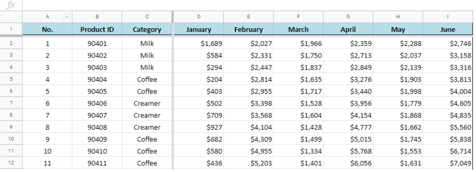 Figure 22. Freeze columns in Google sheets by dragging gray bar
Row 1 and columns A to C are now frozen or locked.
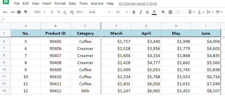 Figure 23. Freeze panes in Google sheets using gray bars
Use Freeze Panes in Google sheets toolbar
Depending on the version we are using, Google sheets may offer a different set of options in freezing cells. Nonetheless, the drop-down menu under View tab > Freeze may be similar to the following:
- No rows
- 1 row
- 2 rows
- Up to current row
- No columns
- 1 column
- 2 columns
- Up to current column
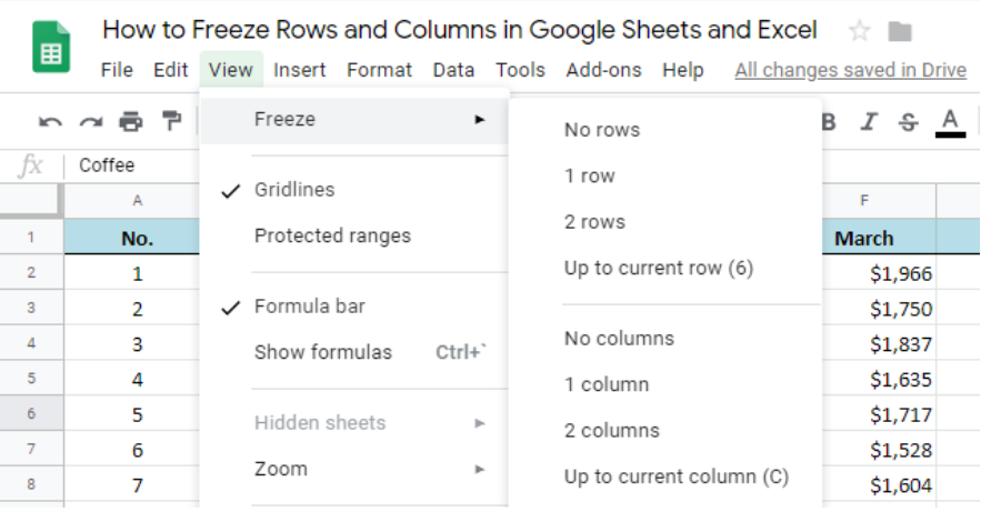 Figure 24. Freeze panes drop-down menu in Google sheets
Google sheet’s toolbar options to freeze 1 row and 1 column have the same use as in Excel’s Freeze Top Row and Freeze First Column.
The no rows and no columns options act similarly as Unfreeze Panes.
Freezing cells in Google sheets are somewhat different because we will have to freeze in two steps: first freeze up to current row, then freeze again up to current column.
In order to freeze the top row and columns A to C like in the previous example, we follow these steps:
Step 1. Select row 1
Step 2. Click the View tab > Freeze > up to current row
 Figure 25. Freeze current row in Google sheets
Step 3. Select column C
Step 4. Click the View tab > Freeze > up to current column
 Figure 26. Freeze current column in Google sheets
As a result, row 1 and columns A to C are now locked and visible even when we scroll down and to the right.
 Figure 27. Freeze multiple rows and columns in Google sheets
How to freeze cells in Excel Mac
Microsoft Excel in Mac works similarly to MS Excel in Windows. The Freeze Panes in Excel Mac offers four options:
- Freeze Panes
- Freeze Top Row
- Freeze First Column
- Unfreeze
 Figure 28. Freeze Panes drop-down menu in Excel Mac
The Unfreeze button is readily available in Mac while in Windows, it only appears after we have locked or frozen some cells. Another difference is that the Freeze Panes button in Excel Mac is under the Layout tab, while the Freeze Panes button in Windows Excel is under the View tab.
The use of the toolbar, however, is the same for both Windows and Mac. In order to freeze the top row in Excel Mac or the first column, we can select any cell and click the freeze button.
How to freeze a row in Excel Mac
In order to freeze a row in Excel Mac, we have to select a row and then click Layout tab > Freeze Panes button > Freeze Panes
 Figure 29. Freeze a row in Excel Mac
How to freeze cells in Excel Mac
In order to freeze multiple rows and columns in Mac, we use the Freeze Panes button. Suppose we want to lock row 1 and columns A to C, we follow these steps:
Step 1. Select cell D2, which is one row after row 1 and one column after column C
Step 2. Click the Layout tab > Freeze Panes button
Step 3. Select the “Freeze Panes” option
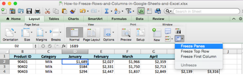 Figure 30. Click Freeze Panes in Excel Mac to freeze cells
We have now successfully locked multiple rows and columns in Mac.
 Figure 31. Freeze multiple rows and columns in Excel Mac
Most of the time, the problem you will need to solve will be more complex than a simple application of a formula or function. If you want to save hours of research and frustration, try our live Excelchat service! Our Excel Experts are available 24/7 to answer any Excel question you may have. We guarantee a connection within 30 seconds and a customized solution within 20 minutes.


Leave a Comment