

By freezing certain areas of our table such as the headers, we can read and navigate around the information in our table with ease. In this tutorial, we will learn how to freeze and unfreeze cells, rows, and columns in Google Sheets.
 Figure 1 – Freeze columns
Freeze columns
- We will select any cell from the column we want to freeze. In this case, we will select Cell A1
- Next, we will go to View and select freeze. Now, we will select the number of columns we want to lock.
 Figure 2 – How to freeze multiple rows
- As we can see, it is possible to freeze any number of columns. However, we have to make sure the screen is wide to show all of them at once. Now, we will click 2 columns
 Figure 3 – Freezing columns
- We will move our cursor to the right border of the grey box that joins the rows and columns. When the hand icon surfaces, we will click on it and drag the borderline that appear on one or more column to the right. This increases the number of columns we want to lock. Now, we will be able to lock Column A to C
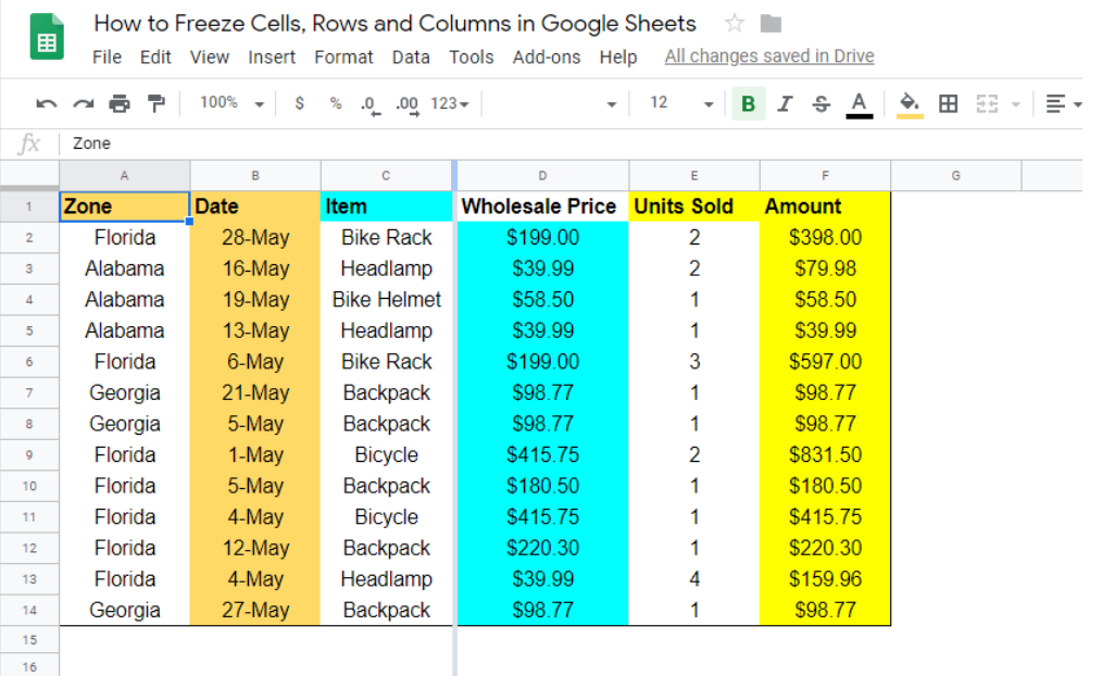 Figure 4 – How to freeze a column
- All columns to the left of the gray line will remain locked as displayed in the figure below.
 Figure 5 – Freeze column
Freeze rows
- We will highlight the row we want to freeze. In this case, we will highlight Cell A1 again.
- Now, we will go to View and select Freeze. Here, we will select the number of rows we want to lock
 Figure 6 – Freezing rows
- We will place our cursor around the right border of the grey box that joins the rows and columns to see the hand icon. Once we have the hand icon, we will click and drag across the number of rows we want to lock.
 Figure 7 – Lock row formula
- Now, whenever we scroll downwards, Row 1 and 2 will remain locked and visible
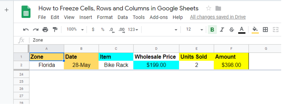 Figure 8 – Results of freezing cells
How to unfreeze columns and rows
- We will go to the View menu
- Next, we will point our mouse to freeze rows…. Or Freeze columns
- We will either select no frozen rows or no frozen columns.
 Figure 9 – How to unfreeze columns
Instant Connection to an Excel Expert
Most of the time, the problem you will need to solve will be more complex than a simple application of a formula or function. If you want to save hours of research and frustration, try our live Excelchat service! Our Excel Experts are available 24/7 to answer any Excel question you may have. We guarantee a connection within 30 seconds and a customized solution within 20 minutes.


Leave a Comment