Excel formula: Calculate cumulative loan interest

Calculate cumulative loan interest

Excel allows a user to calculate a cumulative loan interest, by using the CUMIPMT function. This step by step tutorial will assist all levels of Excel users in calculating a cumulative loan interest.

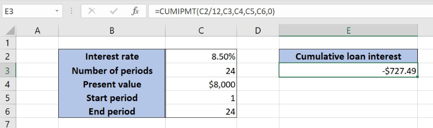Figure 1. The result of the CUMIPMT function

Syntax of the CUMIPMT Formula

The generic formula for the CUMIPMT function is:

=CUMIPMT(rate, nper, pv, start_period, end_period, type)

The parameters of the CUMIPMT function are:

rate – an interest rate for the period (the annual rate divided by 12)
nper – the total number of payments for a loan
pv – the present value of a loan
start_period – a start period of a loan
end_period – an end period of a loan
type – specifies when the payments are made: at the end of a period (0) or at the beginning of a period (1).

Setting up Our Data for the CUMIPMT Function

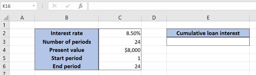Figure 2. Data that we will use in the CUMIPMT example

Let’s look at the structure of the data we will use. In the cell C2, we have the annual interest rate for the loan. In the cell C3, is the total number of payments, while in the C5 is the present value of the loan. Cells C5 and C6 contain the start and end period. We want to get the result of the CUMIPMT function in the cell E3.

Calculate the Cumulative Loan Interest Using the CUMIPMT

In our example, we want to get the cumulative loan interest for the whole period of the loan in the cell E3. Because of that the start period is 1 and the end is 24. The interest rate is 8.50% and the present value of the loan is $8,000.

The formula looks like:

=CUMIPMT(C2/12 ,C3, C4, C5, C6, 0)

The parameter rate is C2/12, as we must pass the monthly interest rate to the function. The nper is the cell C4 (24), while the start_period is C5 (1) and the end_period is C6 (24). The pv is in the C5 ($8,000). The type is 0, as the payments are being made at the end of the period.

To apply the CUMIPMT function, we need to follow these steps:

Select cell E3 and click on it
Insert the formula: =CUMIPMT(C2/12 ,C3, C4, C5, C6, 0)
Press enter

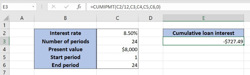Figure 3. Using the CUMPIPMT function to calculate the cumulative loan interest

Finally, the result in the cell E3 is -727.49, which is the cumulative loan interest. The result is always negative, as it is the payment.

Most of the time, the problem you will need to solve will be more complex than a simple application of a formula or function. If you want to save hours of research and frustration, try our live Excelchat service! Our Excel Experts are available 24/7 to answer any Excel question you may have. We guarantee a connection within 30 seconds and a customized solution within 20 minutes.

Did this post not answer your question? Get a solution from connecting with the expert.

Another blog reader asked this question today on Excelchat:

Enter a function in cell G12, based on the payment and loan details, that calculates the amount of cumulative interest paid on the first payment. Be sure to use the appropriate absolute, relative, or mixed cell references.

An Excelchat Expert solved this problem in 13 mins!

Create a formula that calculates total amount of interest saved in the life of the loan when additional payments are made. Formula must correctly calculate interest saved for all periods in the loan (basically, the formula must be accurate when applied to all 360 rows in the amortization schedule.)

An Excelchat Expert solved this problem in 25 mins!

Calculate, in cell D20, the interest amount for period 1 by multiplying the balance in period 0 (cell F19) by the loan interest rate (cell C13) divided by 12. Dividing the interest rate by 12 results in the monthly interest rate. This formula is reusable. The interest for a given period is always the monthly interest rate times the balance from the previous period. [3 points]

An Excelchat Expert solved this problem in 16 mins!