

Excel allows a user to create an annual compound interest schedule, using the simple formula. This step by step tutorial will assist all levels of Excel users in creating annual compound interest schedule
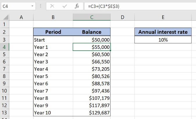 Figure 1. The result of the formula
Syntax of the Formula
The generic formula is:
=initial_balance + ( initial_balance * interest_rate )
The parameters of the formula are:
- initial_balance – an initial balance for calculating the ending balance. The initial balance for every period is the ending balance from the previous period
- interest_rate – an annual interest rate of a loan.
Setting up Our Data for Creating Annual Compound Interest Schedule
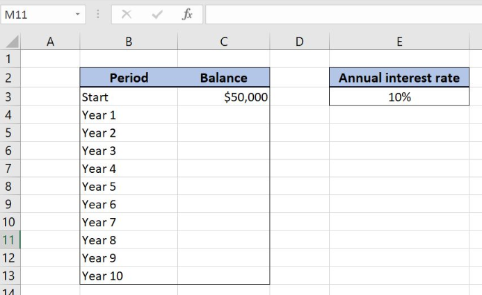 Figure 2. Data that we will use in the example
Let’s look at the structure of the data we will use. In column B, we have the period. In column C, we have the initial balance and want to calculate the balance for each period. In the cell E3, we have the annual interest rate.
Calculating the Annual Compound Interest Schedule
In our example, the initial balance is $50,000 in the cell C3, while the annual interest rate is 10%. Based on these two values, we want to calculate the balance for each period in column C.
The formula looks like:
=C3 / (C3 * $E$3)
The parameter initial_balance is C3, while the interest_rate is in $E$3. Note that we need to fix the cell E3, as the interest rate is the same for all the periods. The initial_balance for every period is the balance from the previous period.
To apply the formula, we need to follow these steps:
- Select cell C4 and click on it
- Insert the formula:
=C3/(C3*$E$3) - Press enter
- Drag the formula down to the other cells in the column by clicking and dragging the little “+” icon at the bottom-right of the cell.
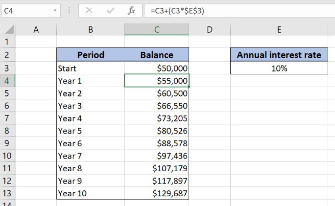 Figure 3. Calculating the annual compound interest schedule
The result in the cell C4 is $50,000, which is the balance for the first year ending, based on input parameters.
Most of the time, the problem you will need to solve will be more complex than a simple application of a formula or function. If you want to save hours of research and frustration, try our live Excelchat service! Our Excel Experts are available 24/7 to answer any Excel question you may have. We guarantee a connection within 30 seconds and a customized solution within 20 minutes.


Leave a Comment