

As we work with Excel, a time comes when we are required to create a chart and keep updating it from time to time. And every time we update the chart, we shall be updating it manually, which becomes a little bit boring. When we know that we shall be updating the data more often, then the best thing to do is to create a dynamic chart range. In this post, we shall learn how to change the range of a graph dynamically.
Creating a dynamic graph
To better understand how a dynamic chart works, it is better to first create it. For you to create a functional dynamic chart, follow the steps below;
The first thing we need to do to create a dynamic chart in Excel 2013 or any other version is to press Ctrl + F3. This will open the Excel Name Manager, then click New button. Alternatively, we can click on the Define Name in the Formula tab under Names Group.
After that, you will be presented with a New Name dialog box. In the dialog box, you will be required to specify the name for your dynamic range in the name box, the name’s scope in the Scope dropdown and OFFSET COUNTA or INDEX COUNTA formula in the Refers to box.
Once you have specified the details above, click OK to proceed.
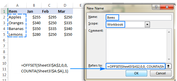 Figure 1: Creating a dynamic chart
Using OFFSET formula to define dynamic named range
We can use an OFFSET function in order to define a chart data range. The OFFSET formula will look as the one below;
=OFFSET(first_cell, 0, 0, COUNTA(column), 1)
In the formula;
- First_cell- refers to the first term that should be included in the dynamic named range
- Column– refers to an absolute reference to the column.
The COUNTA function is essential in this formula as it helps us get number of non-blank cells in the column we are referring to. The number of non-blank cells will be used in the height argument of the OFFSET function and it tells it the number of rows that it should return.
Let us look at an example;
Let us say we want to build a chart dynamic range for column A in sheet 2 and cell A4. We shall use the formula below;
=OFFSET (Sheet2! $A$4, 0, 0, COUNTA (Sheet2! $A: $A), 1)
But if we are to define a dynamic range for our current sheet, then we shall not be obliged to include the sheet name on the references.
Using the INDEX formula to create a dynamic charts
Apart from the above process, we can also prepare a chart data range using the INDEX formula. The INDEX formula utilizes the COUNTA function together with the INDEX function.
The general formula of this formula is as below’
=first_cell: INDEX (column, COUNTA (column))
Notice that this formula has got two parts;
On the left of the operator (:) we have a hard-coded starting reference. This is a reference that we want to start with, like $A$3.
On the right of the operator, we have the INDEX function. This helps us to figure out the ending reference. On this side, we shall be required to supply a whole column for the array and then use COUNTA to get number of row.
Using figure 1 above as an example we shall have the formula as;
=$A$2: INDEX ($A: $A, COUNTA ($A: $A))
In this example, COUNTA will return 5 as non-blank cells in columns A. INDEX will, on the other hand, return $A$5 as the last used cell in column A. thus, our final result shall be $A$2: $A$5.
Note that we have $A$2 as our starting point in the range.
Example 1
Now that we have created our dynamic chart, we need to try it out with new figures. Using a data, let us add an item and see if the dynamic chart will change automatically.
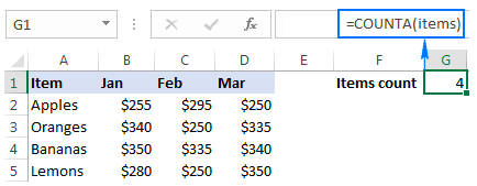 Figure 2: Example of a dynamic chart
Note that in the above dynamic chart, we only have 4 items. Now, let us add one more item to the dynamic range chart and see if it will update.
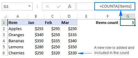 Figure 3: Testing the dynamic chart
When we add one more item, notice how the range of chart changes, we now have 5 items as the items count.
Instant Connection to an Excel Expert
Most of the time, the problem you will need to solve will be more complex than a simple application of a formula or function. If you want to save hours of research and frustration, try our live Excelchat service! Our Excel Experts are available 24/7 to answer any Excel question you may have. We guarantee a connection within 30 seconds and a customized solution within 20 minutes.


Leave a Comment