

Lookup is one of the mostly performed tasks in Microsoft Excel. We often require to perform lookups on different data. Sometimes, the result needs to be an entire row. The combination of the INDEX and MATCH functions allow us to lookup an entire row. In this tutorial, we will learn how to lookup an entire row in Excel.
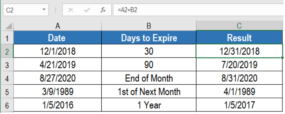 Figure 1. Example of How to Calculate Expiration Dates in Excel
Generic Formula
=Date+Days
Setting up Data
The following example contains some sample dates and days to expiration. Column A,and b has these dates and days.
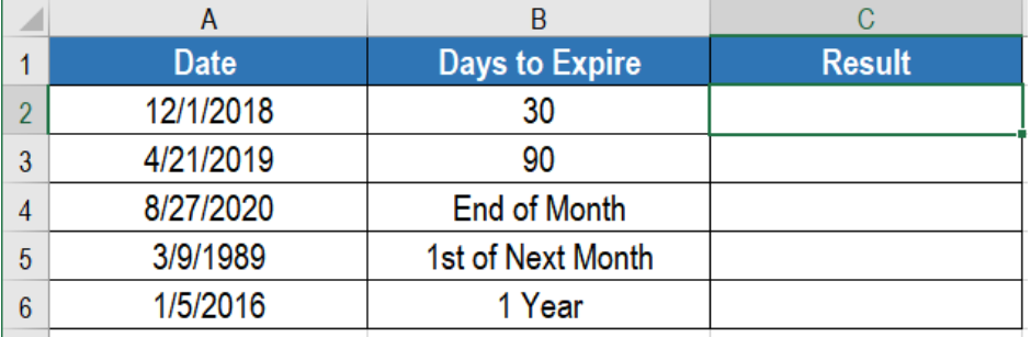 Figure 2. The Sample Data Set
Process
We can use the following formulas to calculate the expiration dates in column C.
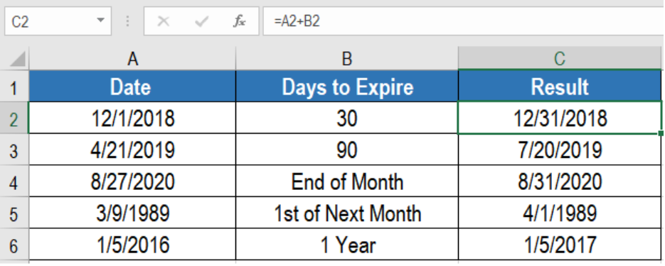 Figure 3. Applying the formulas
=A2+B2
We use this for the dates in A2 and A3. The generic formula uses a simple addition of the days with the date given. We can use other functions to calculate the expiration date as well. Excel processes dates as serial numbers. According to this system, January 1, 1900 has the serial number 1. Continuing the numbers, January 1, 2050 is the serial number 54,789.
=EOMONTH(A4,0)
We can use the EOMONTH function to get the last day of the month. It returns the months in the future or past.
=EOMONTH(A5,0)+1
We can use the EOMONTH function to calculate the first day of the month as well. All we have to do is to use EOMONTH to get the last day of the previous month. Then we add 1 with it.
=EDATE(A6,12)
We can use the EDATE function to calculate expiration dates by months. EDATE returns the same date and months ahead or before.
This will show the expiration dates in column C.
Most of the time, the problem you will need to solve will be more complex than a simple application of a formula or function. If you want to save hours of research and frustration, try our live Excelchat service! Our Excel Experts are available 24/7 to answer any Excel question you may have. We guarantee a connection within 30 seconds and a customized solution within 20 minutes.


Leave a Comment