Excel can calculate a time difference using the TEXT function or by subtracting the times. This step by step tutorial will assist all levels of Excel users in calculating a time difference.

Figure 1. Final result
Syntax of the TEXT formula
=TEXT(value, format_text)
The parameters of the TEXT function are:
- value – a value which we want to format
- format_text – a formatting which we want to apply on the value.
Setting up Our Data for the Time Difference Calculation
Our table consists of 3 columns: “Start Time” (column B), “End Time” (column C) and “Time Difference” (column D). In column D, we want to get a time difference between a start and end time.
 Figure 2. Data that
 we will use in the time difference calculation
Time Difference Calculation Using the TEXT Function
In our example, we want to calculate the time difference between 6:19:00 PM and 3:14:30 PM and get the value in the cell D3.
Formula:
=TEXT(B3-C3,"h:mm:ss")
The value is B3-C3, which Excel calculates as a decimal number. In order to present it as a time, we need to format the value as “h:mm:ss”. This will be our format_text parameter in the function. Setting the time like this, we will get the time difference in hours, minutes and seconds.
Similarly, in the cell D4, we want to get the difference in hours and minutes, so format_text parameter will be “h:mm”. Finally, in the cell D5, we want only hours, so the format_text will be “h”.
To apply the TEXT function, we need to follow these steps:
- In cell D3, insert the formula:
=TEXT(B3-C3,"h:mm:ss") - Select cell D4 and click on it
- In cell D4, insert the formula:
=TEXT(B4-C4,"h:mm") - In cell D5, insert the formula:
=TEXT(B5-C5,"h")
 Figure 3. Using the TEXT function to calculate the time difference
We can see in cell D3, we get the difference 3:04:30, which is “h:mm:ss” format. In the cell D4 we get 3:04 (“h:mm”), while in the cell D5 we get the difference only in hours (3), which is “h” format.
Subtract Times to Calculate a Time Difference
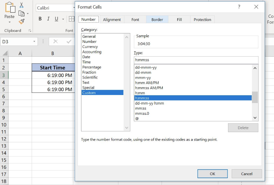
Another way to calculate a time difference is to simply subtract two cells containing time values. We will use the same data set like in the previous example. Before doing the calculation, we must set the format of the resulting cell as a time. To do this, we need to press Ctrl+1, choose “Custom” category and enter the format of the time – h:mm:ss.
 Figure 4. Formatting the cells for times subtraction
Formula:
B2-C2
Similarly to the previous example, in the cell D4, we want to get the difference in hours and minutes, so the format will be “h:mm”, while in the cell D5, we want only hours, so the format will be “h”.
To subtract the times, we need to follow these steps:
- Select cell D3 and click on it
- Press Ctrl+1
- Choose “Custom” category and enter the format of the time – h:mm:ss
- Insert the formula: =B3-C3
- Press enter
- Select cell D4 and click on it
- Press Ctrl+1
- Choose “Custom” category and enter the format of the time – h:mm
- Insert the formula: =B4-C4
- Press enter
- Select cell D5 and click on it
- Press Ctrl+1
- Choose “Custom” category and enter the format of the time – h
- Insert the formula: =B5-C5
- Press enter
 Figure 5. Subtract the times to get the times difference
As a result, we get the same times as in the previous example.
Most of the time, the problem you will need to solve will be more complex than a simple application of a formula or function. If you want to save hours of research and frustration, try our live Excelchat service! Our Excel Experts are available 24/7 to answer any Excel question you may have. We guarantee a connection within 30 seconds and a customized solution within 20 minutes.


Leave a Comment