

The usage of the COUNTIF & Conditional Formatting functions in Excel can yield useful and visually appealing results. This step by step tutorial will assist all levels of Excel users in creating dynamic conditional formats.
Our data-set shows the date and the type of vehicle rented. Now, we want to show the overall count of a type of vehicle with color coding.
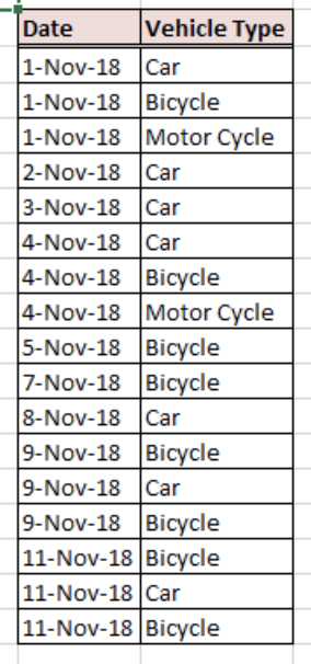 Figure 1: Dataset containing Date and Vehicle Type
Usage of the “COUNTIF” Excel Function
Syntax of the COUNTIF Formula: COUNTIF(range, criteria)
We are going to apply the COUNTIF function to count the number of vehicles sold by type in the first 11 days of November. We have three types of vehicles – “Car”, “Motorcycle” and “Bicycle”.
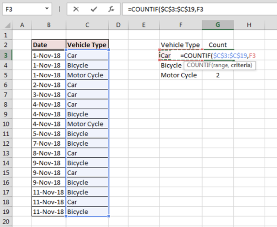 Figure 2: Usage of the COUNTIF Formula on the given dataset
- We will calculate the number of vehicles within each type in cells G3 to G5, using the “COUNTIF” formula
- We will break down the COUNTIF formula in cell G3 as below:
= COUNTIF($C$3:$C$19,F3) - The range C3:C19 refers to our dataset that elaborates the type of vehicle rented out on a given date
- F3 refers to the vehicle type that we would like to count, “Car” in this case
We can apply the same formula for the “Bicycle” and “Motorcycle” categories in cells G4 and G5 respectively. The results can be seen in the figure below.
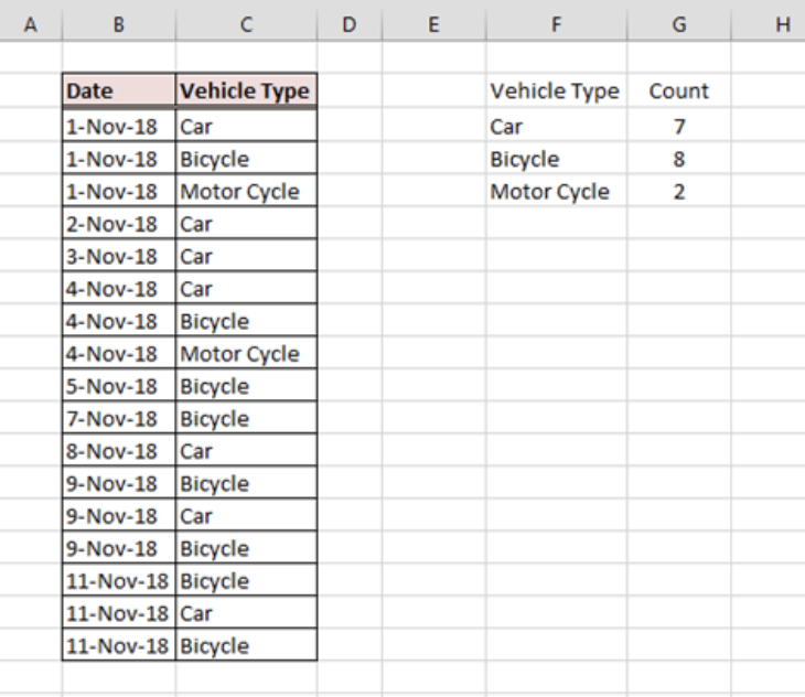 Figure 3: COUNTIF result
Implementation of Conditional Formatting
Now, we will apply conditional formatting to the cells that contain the COUNTIF formula.
Conditional formatting helps us identify the least and most rented vehicle.
The application of the conditional formatting is discussed in the steps below:
- Select cells G3:G5
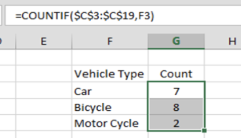 Figure 4: Cell Selection for Conditional Formatting
- Go to Home > Conditional Formatting and click the small drop down menu adjacent to conditional formatting
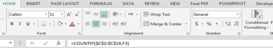 Figure 5: Selection of Conditional Formatting from Home
- Select the preferred Color Scale
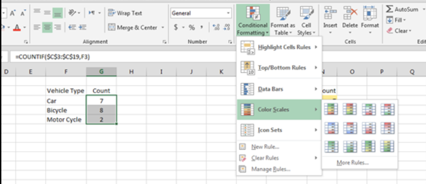 Figure 6: Selection of Color Scale
- Select any option in Color Scale and the cells containing the COUNTIF formula will be highlighted based on the selected option.
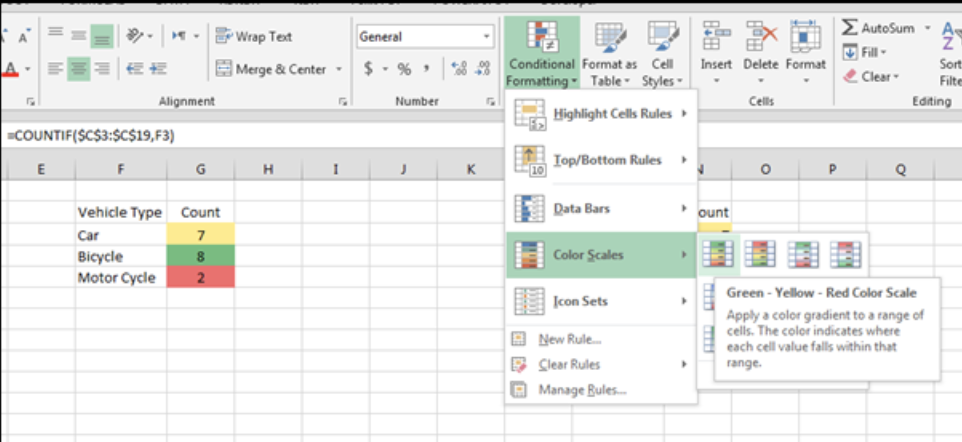 Figure 7: Application of Conditional Formatting
Combining Excel functions together can help us solve complex tasks quickly.
The final result will be:
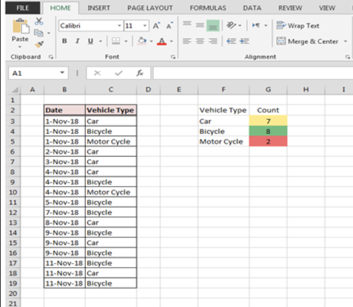 Figure 8: Final Result


Leave a Comment