

We can count unique text values in a range by using a combination of FREQUENCY, MATCH, ROW and SUMPRODUCT functions. We can also achieve the same result with the COUNTIF function. The steps below will walk through the process.
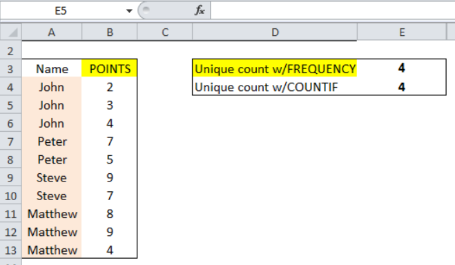 Figure 1: Result of Count of Unique Text Values in a Range
General formula
=SUMPRODUCT(--(FREQUENCY(MATCH(txt,txt,0),ROW(txt)-ROW(txt.firstcell+1)>0))
”txt” is the range containing the text or names
Formula
=SUMPRODUCT(--(FREQUENCY(MATCH(A4:A13,A4:A13,0),ROW(A4:A13)-ROW(A4)+1)>0))
Setting up the Data
We will set up the table as shown in figure 2 with hypothetical players who have scored some points. Now, we have players whose names have appeared more than once. Our intention is to count the number of unique names that appear.
- We will input the names in range A4:A13
- The points will be placed in Column B
- Cell E3 and Cell E4 will contain the results by applying the FREQUENCY and COUNTIF functions respectively
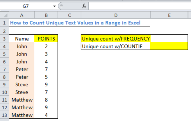 Figure 2: Setting up the Data
Applying the Frequency Function
- We will insert the formula below into Cell E3
=SUMPRODUCT(--(FREQUENCY(MATCH(A4:A13,A4:A13,0),ROW(A4:A13)-ROW(A4)+1)>0))
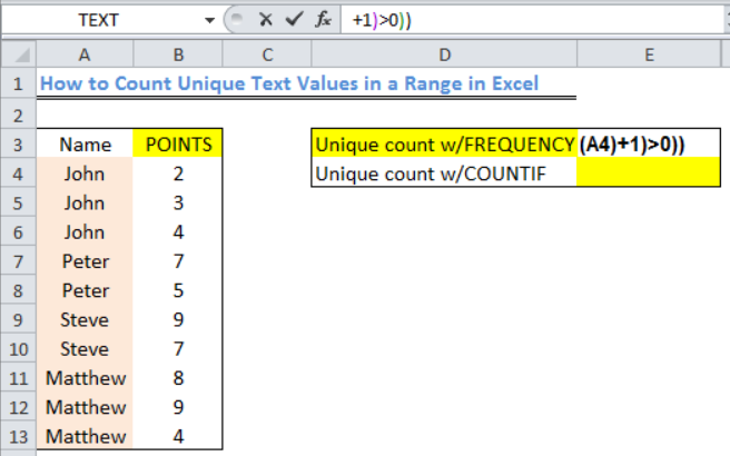 Figure 3: How to Count Unique Text Values in a Range
- We will press the enter key
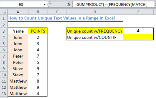 Figure 4: Result of Unique Text Values in the Range
Applying the COUNTIF Function
- We will insert the formula below into Cell E4
=SUMPRODUCT(1/COUNTIF(A4:A13,A4:A13))
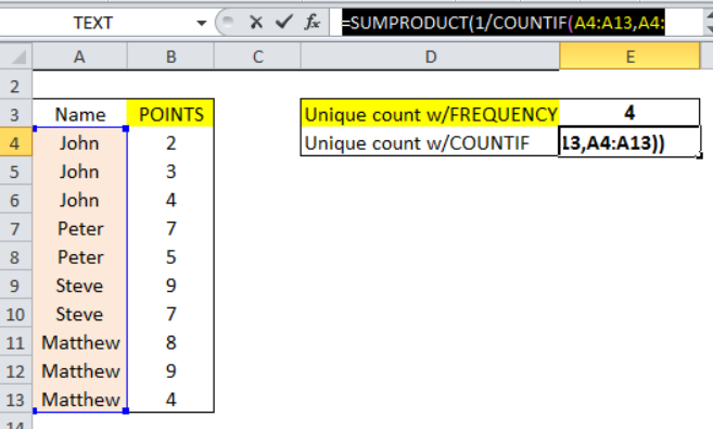 Figure 5: How to Count Unique Text Values in a Range with the COUNTIF function
- We will press the enter key
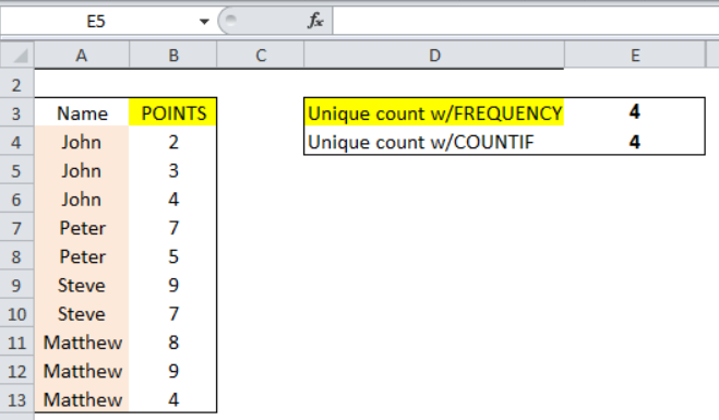 Figure 6: Result of Count of Unique Text Values in a Range
Explanation
=SUMPRODUCT(--(FREQUENCY(MATCH(A4:A13,A4:A13,0),ROW(A4:A13)-ROW(A4)+1)>0))
- MATCH Function
This function gets the position of each name in the range. MATCH only returns the position of the first match in the range, as a result, any name that appears more than once will bear the same number so that the returned array of this example looks like this:
{1;1;1;4;4;6;6;8;8;8}
- ROW Function
ROW(A4:A13)-ROW(A4)+1
The argument above is used to build a straight and sequential array. This is achieved by using the row number of each item in the range and the first item in the range. The returned array will look like this:
{1;2;3;4;5;6;7;8;9;10}
- FREQUENCY Function
The FREQUENCY function does not work with non-numeric data; hence, the bulk of the formula will convert the data into numeric data that FREQUENCY works with.
The FREQUENCY function uses the array supplied by MATCH and that supplied by ROW.
The FREQUENCY function will return an array of values that shows the count for every value that is present in the array. FREQUENCY will return zero for any number that repeats itself in the array. The resultant array will look like this:
{3;0;0;2;0;2;0;3;0;0;0}
- SUMPRODUCT Function
The returned array from FREQUENCY is evaluated by TRUE or FALSE to know if the numbers are greater than zero. Afterward, TRUE values are returned as 1 and FALSE as 0. The resultant array in SUMPRODUCT will look like this:
{1;0;0;1;0;1;0;1;0;0;0}
SUMPRODUCT then sums the values and the result is 4 as shown.
Instant Connection to an Expert through our Excelchat Service
Most of the time, the problem you will need to solve will be more complex than a simple application of a formula or function. If you want to save hours of research and frustration, try our live Excelchat service! Our Excel Experts are available 24/7 to answer any Excel question you may have. We guarantee a connection within 30 seconds and a customized solution within 20 minutes.


Leave a Comment