

While working with Excel, we are able to count unique numeric values in a data set by using the SUM, FREQUENCY and IF functions, with some help using the double negative “—”. This step by step tutorial will assist all levels of Excel users in counting unique numeric values based on a criteria.
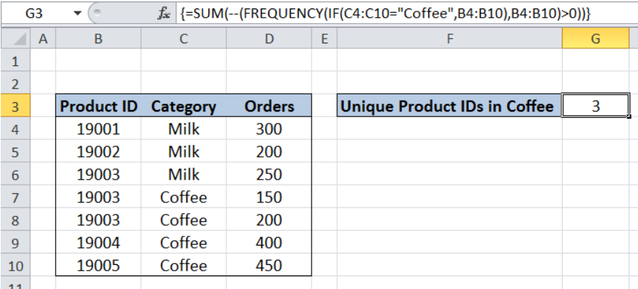 Figure 1. Final result: Count unique numeric values with criteria
Final formula: {=SUM(--(FREQUENCY(IF(C4:C10="Coffee",B4:B10),B4:B10)>0))}
Syntax of SUM Function
SUM adds all given values
=SUM(number1,[number2],...])
- number1 – any number, array or cell reference whose values we want to add
- Only number1 is required; succeeding numbers are optional
Syntax of the FREQUENCY function
FREQUENCY determines how often values occur within a range, and returns a vertical array of numbers. Since FREQUENCY returns an array, it must be entered as an array formula.
FREQUENCY automatically returns zero for numbers that appear more than once in the data array
=FREQUENCY(data_array, bins_array)
- data_array – an array or reference to a set of values whose frequencies we want to count
- bins_array – an array or reference to intervals specifying how we want to group the values in data_array
- FREQUENCY ignores blank cells
Syntax of IF Function
IF function evaluates a given logical test and returns a TRUE or a FALSE
=IF(logical_test, [value_if_true], [value_if_false])
- The arguments “value_if_true” and “value_if_false” are optional. If left blank, the function will return TRUE if the logical test is met, and FALSE if otherwise.
Setting up Our Data
Our table contains three columns: Product ID (column B), Category (column C) and Orders (column D). We want to determine the number of unique Product IDs in the category “Coffee” and record it in cell G3.
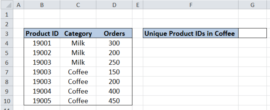 Figure 2. Sample data to count unique numeric values with criteria
Count unique Product IDs in Coffee
In order to count unique Product IDs in Coffee, we follow these steps:
Step 1. Select cell G3
Step 2. Enter the formula: =SUM(--(FREQUENCY(IF(C4:C10="Coffee",B4:B10),B4:B10)>0))
Step 3: Press Ctrl + Shift + Enter
FREQUENCY returns an array so our formula needs to be entered as an array formula by pressing Ctrl + Shift + Enter.
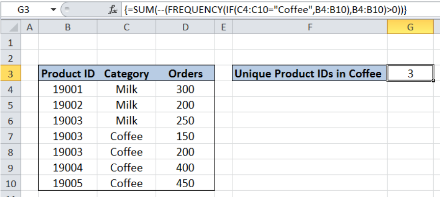 Figure 3. Entering the formula using SUM, FREQUENCY and IF
=SUM(--(FREQUENCY(IF(C4:C10="Coffee",B4:B10),B4:B10)>0))
Our data_array for FREQUENCY is the IF function IF(C4:C10="Coffee",B4:B10). IF returns the value in column B if the category in column C is “Coffee”. The result is an array like this:
{FALSE;FALSE;FALSE;19003;19003;19004;19005}
The FREQUENCY function then returns the number of times a value occurs in the array. However, it automatically returns a zero for values occurring more than once. The resulting array is:
{0;0;0;2;0;1;1}
The array is then tested to be greater than zero.
{FALSE;FALSE;FALSE;TRUE;FALSE;TRUE;TRUE}
The double negative sign “–” converts the values TRUE and FALSE into 1 and 0, respectively.
The array becomes: {0;0;0;1;0;1;1}
Finally, the result in cell G3 is the sum of the values in the array which is 3. There are three unique Product IDs with the category “Coffee”: 19003, 19004 and 19005.
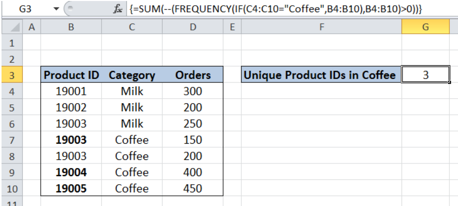 Figure 4. Output: Count unique numeric values with criteria
Most of the time, the problem you will need to solve will be more complex than a simple application of a formula or function. If you want to save hours of research and frustration, try our live Excelchat service! Our Excel Experts are available 24/7 to answer any Excel question you may have. We guarantee a connection within 30 seconds and a customized solution within 20 minutes.


Leave a Comment