

Excel now supports millions of rows. It is easy to get lost working with large datasets to figure out the meaning of the values. Repeating header rows can help us with this problem. In this tutorial, we will learn how to keep the top line visible in Excel.
Excel Repeat Header Row when Scrolling
We can repeat header rows in Excel using the Freeze Pane options. If we have one row to freeze, we can use the Freeze Top Row to modify the worksheet so the first row is always visible. In other cases where we have multiple header rows, we can use the Freeze Panes option. This helps us in Excel to always show the top row.
How to Make Column Headers Scroll in Excel Using Freeze Top Row
We use a student information database in this example. Column A, B, and C has the names, IDs and ages.
 Figure 1. The Sample Data Set
To Repeat row when scrolling, we need to:
- Click on cell A1. Drag the selection to cells A1 to A3. These are the labels we want to repeat while scrolling.
- Click on the View tab on the ribbon.
- From here, Click on the arrow next to the Freeze Panes option in the Window group.
- This will open the freezing options. We need to choose to Freeze Top Row.
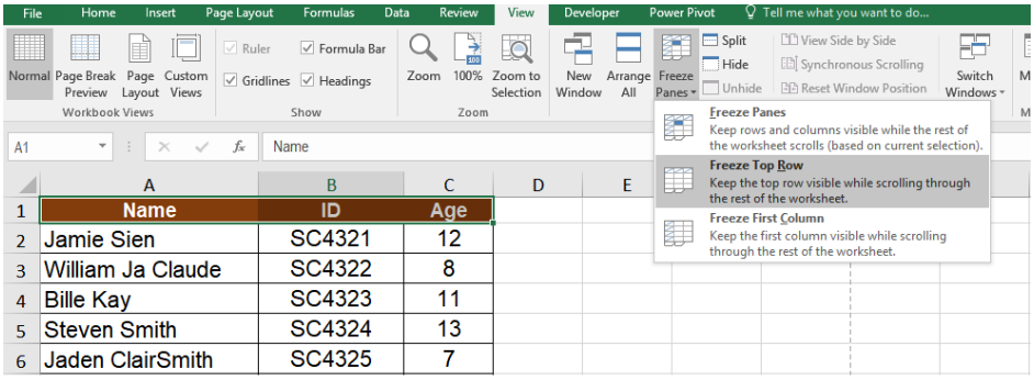 Figure 2. Example of the Freeze Pane Options
This will make the first row always visible in Excel.
 Figure 3. Repeat Header Row When Scrolling with Freeze Top Row
After we Freeze the row, the Freeze Panes option turns into Unfreeze Panes. This is a quick way to unfreeze the row.
 Figure 4. The Unfreeze Panes Option
How to Make a Column Stay in Excel Containing Multiple Header Rows
Sometimes, we may have tables having multiple header rows. These might be a bit different from the usual table structures. But, they help to understand the data clearly. We have to modify the worksheet so the first row is always visible when we scroll the worksheet down. We can achieve that using the Freeze Panes feature.
In this example, we use a student grade database. Column A and B have the details, C has the grades, column D and E contain whether the student has passed or not.
 Figure 5. Data with a Header Containing Two Rows
To freeze the header rows.
- We need to select cell A3.
- Follow steps 1 and 2 from the previous example.
- From here, we need to select the Freeze Panes option. This lets us lock several rows at once.
 Figure 6. Repeat Header Rows with the Freeze Panes Option
Notes
- It is a good habit to unfreeze the rows at first if it does not work.
- When the rows are locked in the table, we will see the Unfreeze Panes option in place of Freeze Panes. It is a good practice to look at the option name at first before attempting to lock or unlock the row.
How to Keep Title Row when Scrolling in Google Sheets
We can repeat header rows when scrolling in Google Sheets using the Freeze option. To lock the first row from the previous example:
- We need to select cells A1 to A3.
- Next, we need to click View.
- From here, we need to click Freeze > 1 Row.
 Figure 7. The Freeze Option in Google Sheets
This will repeat the header row when scrolling in Google Sheets.
 Figure 8. Example of Repeating Header Rows when Scrolling in Google Sheets
We can freeze multiple rows by selecting 2 Rows or Up to current row from the Freeze options.
 Figure 9. Example of repeating 2 rows when scrolling in Google Sheets
Repeating header rows help to work with large datasets without getting lost. The Freeze options help us to repeat header rows in both Excel and Google Sheets. This saves a lot of time and makes working with large datasets comparatively easier.
Instant Connection to an Excel Expert
Most of the time, the problem you will need to solve will be more complex than a simple application of a formula or function. If you want to save hours of research and frustration, try our live Excelchat service! Our Excel Experts are available 24/7 to answer any Excel question you may have. We guarantee a connection within 30 seconds and a customized solution within 20 minutes.


Leave a Comment