

Google Sheets conditional formatting is used to highlight the cells or rows based on condition(s) with the help of built-in rules and custom formula. Mostly, we apply Google Sheets conditional formatting based on another cell value using custom formula rule by comparing it with data set values with the help of logical operators equal to, greater than, less than and so on.
 Figure 1. Conditional Formatting Based on Another Cell
Applying Google Sheets Conditional Formatting Based on Another Cell
We apply Google Sheets conditional formatting based on another cell value containing numbers, text or date with the help of custom formula rule. In this method, we compare the targeted data with another cell value as a condition by choosing the desired formatting style(s) of text color, cell color, etc. For example, we want to highlight the leads data where the worth or value of a lead is Greater Than Equal To (>=) value based on another cell.
Figure 2. Leads Data to Highlight Based on Another Cell 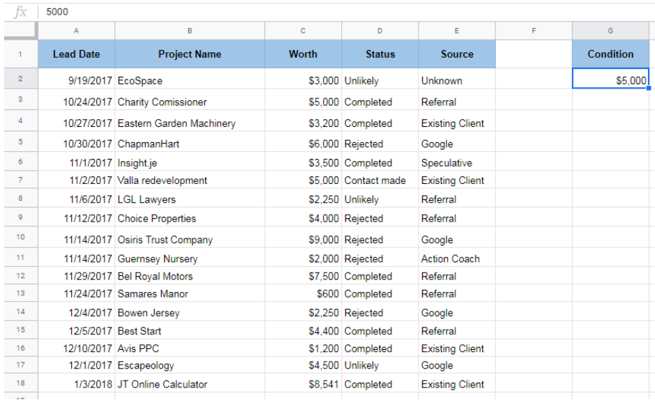
Using a Custom Formula Rule
In Google Sheet Conditional Formatting we create a conditional formatting rule using the Custom Formula Rule option to compare and highlight the data based on another cell value. By using the formula rule we can easily compare and highlight the data as per the selected formatting style. We need to use these steps;
- Select the targeted data values that we need to conditionally format based on another cell value. In our example, we will select values of cells range A2: E18 because we want to highlight these values based on another cell value G2 as a condition.
 Figure 3. Selecting Targeted Data Values
- Go to Format tab and select Conditional Formatting.
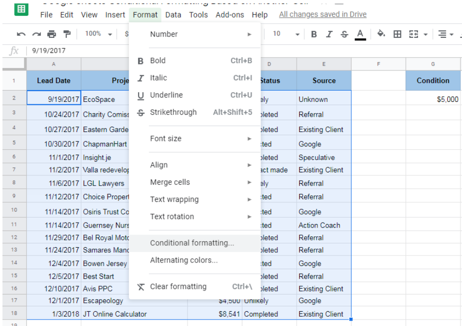 Figure 4. Selecting Conditional Formatting Menu
- From Conditional Format Rules window, select the Custom Formula Is from Format Rules drop-down list.
 Figure 5. Conditional Format Rules
- Under the Custom Formula Is, we need to enter the custom formula in Value or Formula box. In our example, we need to compare the worth amount of leads in column C based on another cell value and want to highlight those leads that are greater than equal to (>=) cell value of G2. Therefore we use the custom formula =$C2>=$G$2.
- We are required to insert the dollar sign ($) to fix the column reference and keep the row reference free to move, like $C2. To freeze the cell reference of another cell value we need to insert the dollar sign with column and row reference both, like $G$2.
 Figure 6. Inserting Custom Formula
- Now we select the Formatting Style from the provided styles of Text Color, Cell Color, Bold, etc as per choice or apply the default one and press Done button. Google Sheets conditional formatting based on another cell will be applied where the given condition meets.
 Figure 7. Google Sheet Conditional Formatting
Instant Connection to an Expert through our Excelchat Service
Most of the time, the problem you will need to solve will be more complex than a simple application of a formula or function. If you want to save hours of research and frustration, try our live Excelchat service! Our Excel Experts are available 24/7 to answer any Excel question you may have. We guarantee a connection within 30 seconds and a customized solution within 20 minutes.


Leave a Comment