How to Highlight Values Between a Range in Excel

We often need to highlight values between a range. It might be needed to put emphasis on a set of values or to represent outliers. We can highlight values between a range in Excel using conditional formatting. It will retrieve specific values from the data based on conditions provided. In this article, we will learn how to highlight values between a range.

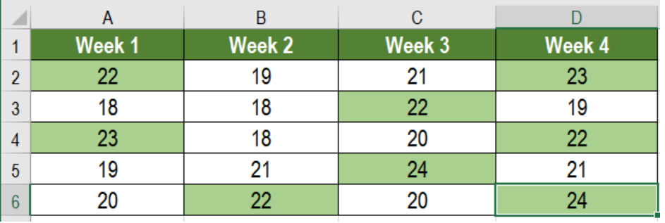Figure 1. Example of How to Highlight Values Between a Range

Generic Formula

=AND (A1>=lower,A1<=upper)

Process

Here, we need to use this formula along with conditional formatting. Excel evaluates this formula for each cell in the range. In the meantime the active cell in the selection is kept relative at the time we create this rule. If we apply this rule to a range, the first cell will be active.The rule is then evaluated for each cell while the first cell is fully relative. The formula uses AND with two conditions. The result will be TRUE when both conditions are met. This will trigger the conditional formatting and highlight the cells.

Setting up Data

The following example uses a temperature data set of twenty days. Column A to D has these temperatures.

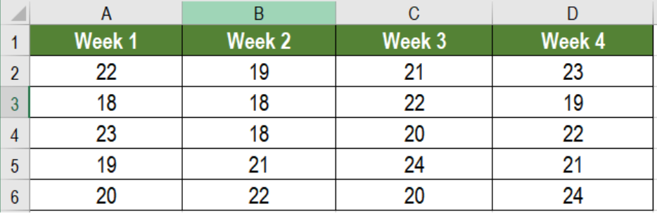Figure 2. The Sample Data Set

To highlight the temperature readings between 22 and 25, we need to

• Select cells A2 to D6 by clicking on A2 and dragging it till D6.
• Go to the home tab in the ribbon. Select Conditional Formatting. Click on New Rule.

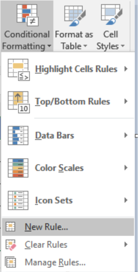Figure 3. Example of how to Apply Conditional Formatting

• Click on Use a formula to determine which cells to format.

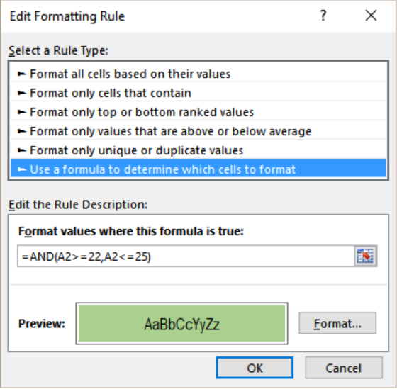Figure 4. Applying the Formula to the Conditional Format

• Click the Format values where this formula is true box. On the formula box, we have to write the formula =AND (A2>=20,A2<=25).  
• Next, we have to select the Format tab near the preview box.
• Then, we have to go to Fill>Background Color and select the color we want to highlight in.  

Figure 5. Managing the Display Options

• Click OK twice.

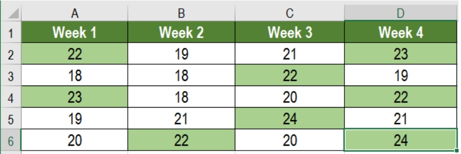Figure 6. The Final Result

This will highlight the temperatures between 22 to 25 in columns A to D.

Most of the time, the problem you will need to solve will be more complex than a simple application of a formula or function. If you want to save hours of research and frustration, try our live Excelchat service! Our Excel Experts are available 24/7 to answer any Excel question you may have. We guarantee a connection within 30 seconds and a customized solution within 20 minutes.