

Excel provides an easy way of highlighting cells based on a given condition or criteria by using conditional formatting. This step by step tutorial will assist all levels of Excel users in highlighting cells that equal to a certain value.
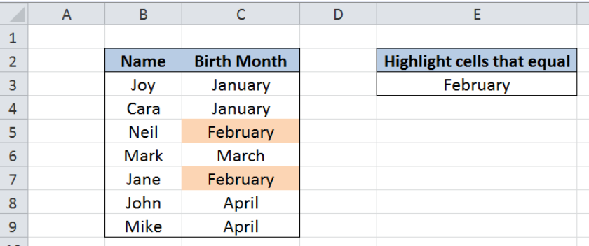 Figure 1. Final result: Highlight cells that equal to a value
Setting up the Data
Our table consists of two columns: Name (column B) and Birth Month (column C). In cell E3, we enter our criteria “February”. We want to use conditional formatting to highlight the cells that equal to the value in cell E3, or “February”.
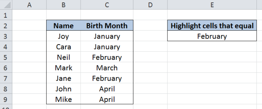 Figure 2. Sample data to highlight cells that equal a value
Highlight cells that equal to cell E3
We want to highlight the cells in column C that equal to the value in cell E3 through conditional formatting. Let us follow these steps:
Step 1. Select the cells we want to highlight. In this case, select cells C3:C9.
Step 2. Click the Home tab, then the Conditional Formatting Menu and select “New Rule”. The New Formatting Rule dialog box will pop up.
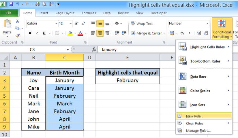 Figure 3. Creation of a new rule in conditional formatting
Step 3. Select the Rule Type “Use a formula to determine which cells to format” and enter this formula in the dialog box : =C3=$E$3
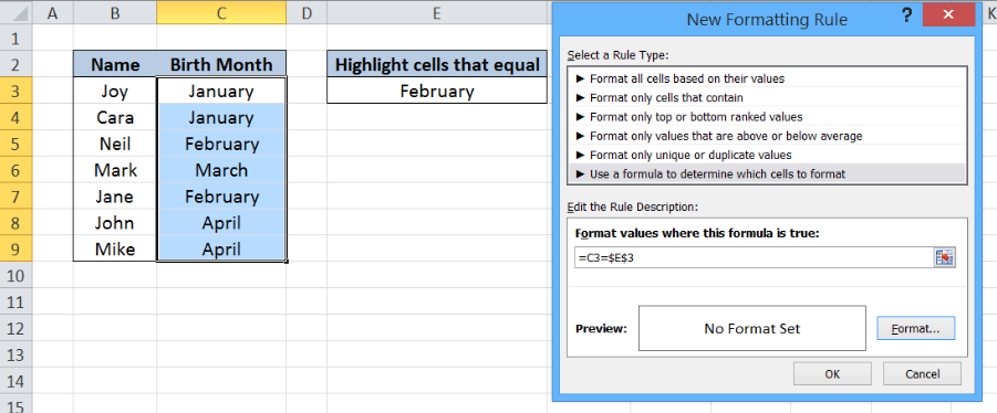 Figure 4. Entering the formula as a condition or formatting rule
Our formula =C3=$E$3 serves as the condition or rule that will trigger the conditional formatting. For every cell in the range C3:C9, if the value is equal to the value in cell E3, which is “February”, the format will be changed.
The dollar sign “$” fixes the cell E3 which is our basis for changing the format of the cells in column C.
To change the format, let us proceed to the next step.
Step 4. Click “Format” and then decide on the new format to apply to the cells in column C. We can change the font, borders or fill the cells with different colors.
Example
Select “Fill” and choose Orange, Accent 6, Lighter 60% and click OK.
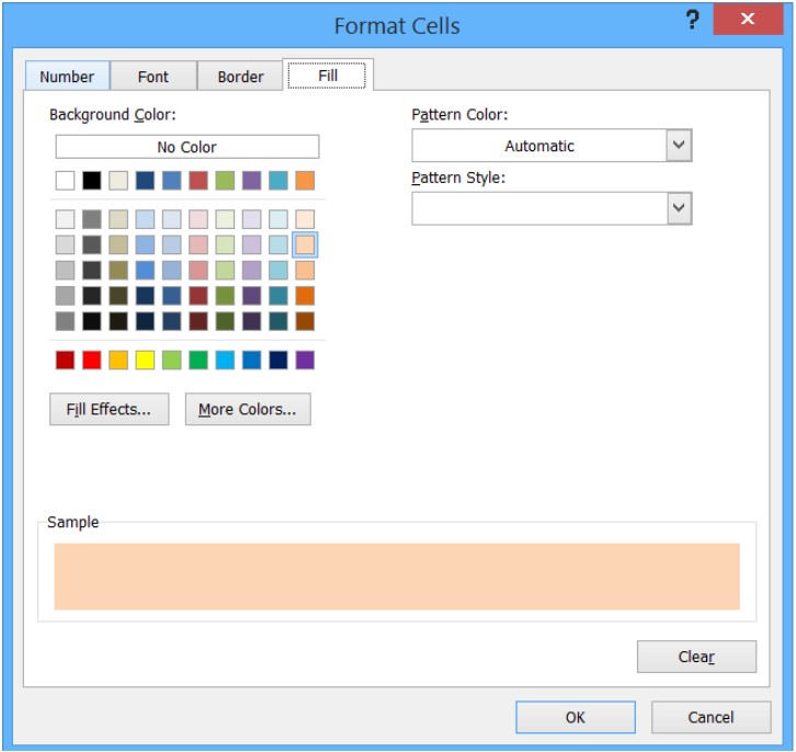 Figure 5. Selection of the format to use
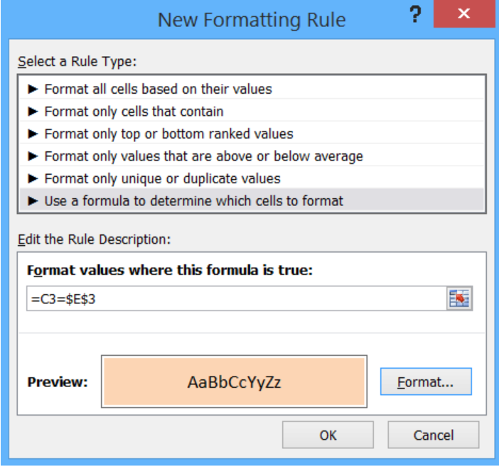 Figure 6. Completion of the new formatting rule with formula and format
This rule highlights the cells that satisfy the condition of C3=E3. As a result, the cells that equal in value to E3 or “February” are highlighted as shown below.
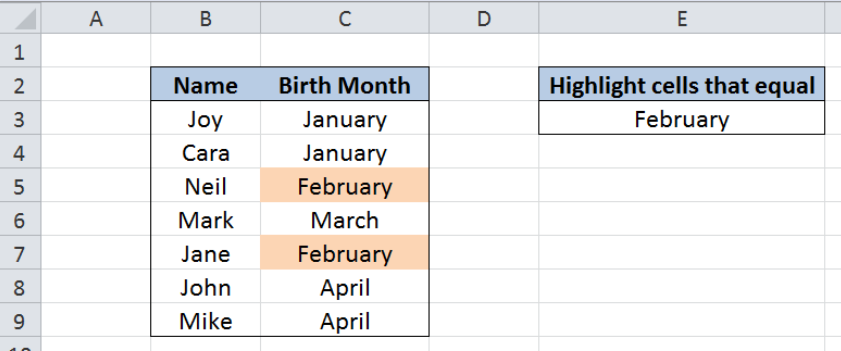 Figure 7. Output: New conditional formatting rule reflected in cells C5 and C7
With conditional formatting, we can now highlight the cells in column C that equal in value to cell E3. Let us try changing the value in E3 to “march”.
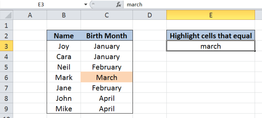 Figure 8. Highlighting cells that equal to “march”
The conditional formatting rule is automatically applied to cell C6 as shown above. By just changing the value of one cell, we can now quickly highlight the specific cells in our worksheet with little effort.
Notes
- The comparison of values is not case-sensitive, since the value in cell E3 is in lowercase while the highlighted value in C6 is in proper case.
- However, we can use the EXACT function to avoid case sensitivity errors. We can enter this formula instead: =EXACT(C3,$E$3)
- In highlighting cells that equal to a value, we can also enter that value directly into our formula in conditional formatting. We can use this formula in our formatting rule:
=C3=”February”
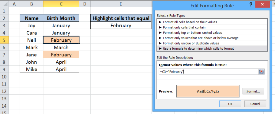 Figure 9. Output: Hardcoding the value “February” into the formatting rule
This method is longer and more tedious but it is also less prone to error. As shown above, the result is the same as in the previous example where the formula we used was: =C3=$E$3.
Most of the time, the problem you will need to solve will be more complex than a simple application of a formula or function. If you want to save hours of research and frustration, try our live Excelchat service! Our Excel Experts are available 24/7 to answer any Excel question you may have. We guarantee a connection within 30 seconds and a customized solution within 20 minutes.


Leave a Comment