

If you need to highlight rows and columns with an approximate match in Excel, then this article will help you in developing an understanding of this. Therefore, the main purpose of this article is to explain how to highlight the match lookup using the conditional formatting tool.
Highlight approximate match lookup using conditional formatting
Highlighting the approximate match lookup using conditional formatting option, also the combination of LOOKUP function and OR function will solve the problem.
Hence, the following formula is generic and will highlight the approximate match lookup values accordingly.
Formula using OR and LOOKUP functions
=OR($Xn=LOOKUP(value1,data1),X$n=LOOKUP(value2,data2))
Explanation of formula
The LOOKUP function can search for a specific value in the array or data. In the above formula, Xn refers to any cell under consideration in the Excel sheet.
In the formula described above, value1 and value2 in the cells are using OR function to lookup with defined criteria, and have conditional formatting. Each cell can have different criteria to format and can be adjusted in the setting.
Example
A two-dimensional array of 6×6 has been considered, which shows row numbers as the parameter width and column number as height. These arrays are named as widths and heights respectively. The entries of the array show the area corresponding to the width and height.
A sample of each, width and height are separate which is then looked for in the 2-D array.
Step 1:
Firstly, let’s have a look at the sample that we will go through in the figure below:
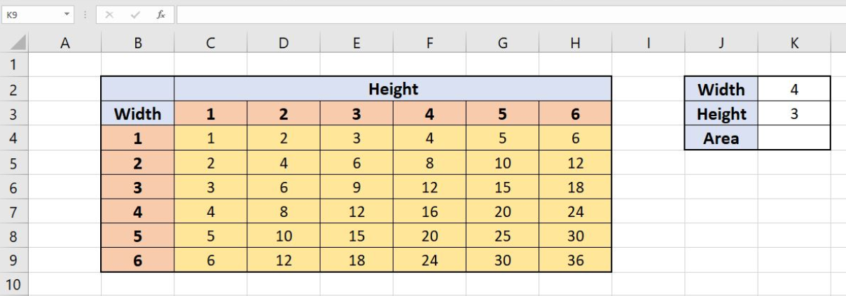 Figure 1. Sample sheet to highlight approximate match lookup conditional formatting
Step 2:
Secondly, in order to calculate the value of the area and making an approximate match, enter the following formula in cell K4:
=INDEX(C4:H9,MATCH(width,widths,1),MATCH(height,heights,1))
INDEX function is basically to retrieve the value of the area corresponding to the entered width and height. MATCH function is used to make an approximate match by setting its 3rd parameter to 1. The two MATCH functions return the row and column number respectively which is used as an address by the INDEX function to retrieve the value in that place in array C4:H9.
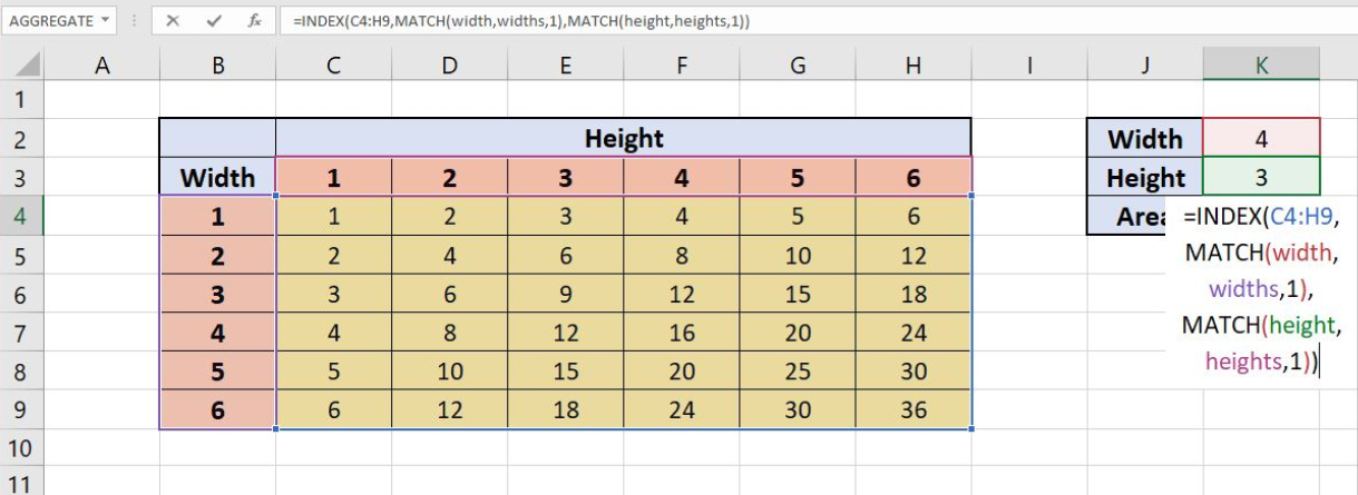 Figure 2. Finding the approximate match from the array
Step 3
Thirdly, select the range of cells (here: B3:H9) and adjust the format setting. After that, go to the Conditional Formatting option in the drop-down menu of Home button (in the menu bar) and click the “Manage Rules” option at the end of the menu.
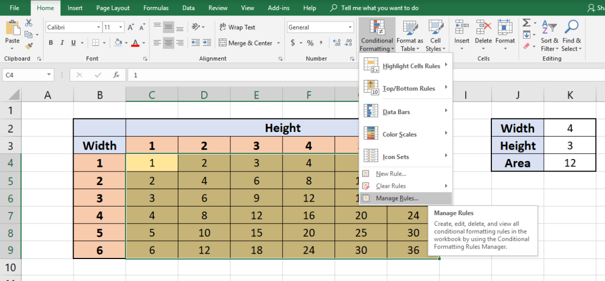 Figure 3. Selecting and Conditional Formatting the cells
Step 4
After that, Conditional Formatting Rules Manager’s pop-up window will appear. Click on the “New Rule” button in this window.
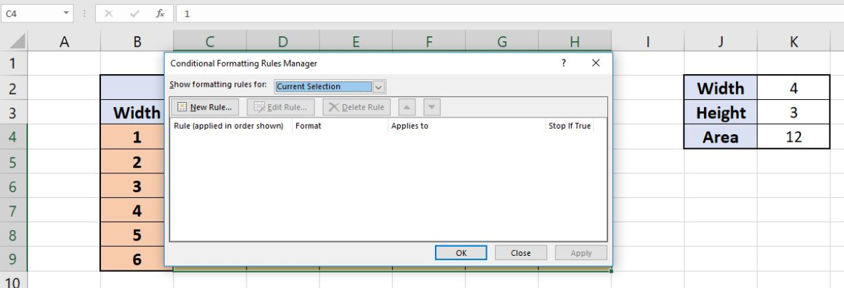 Figure 4. Creating a New Rule from Conditional Formatting Rules Manager
Step 5
Now, another pop-up window will appear to create a new formatting rule of your own. There are several options to create a new rule; select the “Use a formula to determine which cells to format” option from the menu.
As a result, a formula bar will appear in the same pop-up window below those options.
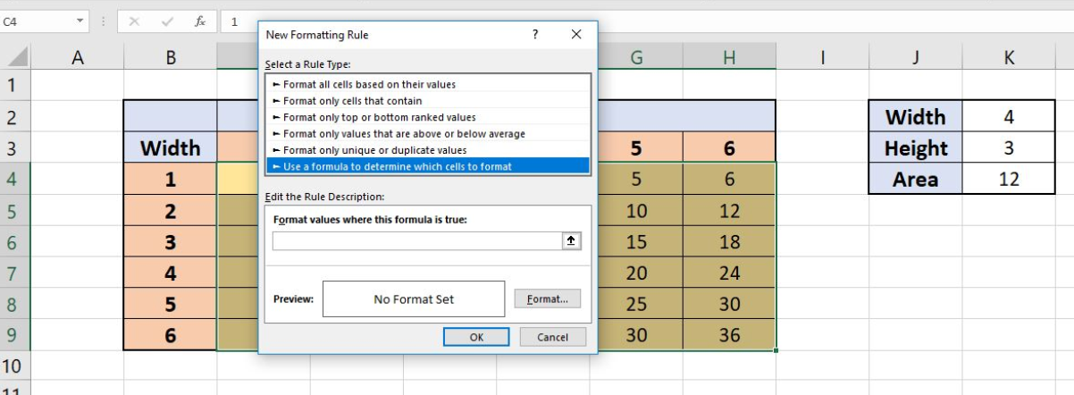 Figure 5. Enter the formula to define which cells to format
Step 6
Let’s enter the formula written below in this formula bar:
=OR($B5=LOOKUP(width,widths),B$5=LOOKUP(height,heights))
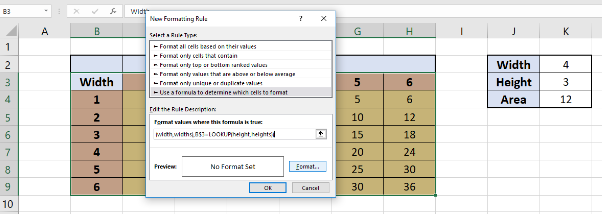 Figure 6. Defining to format the approximate match lookup, in conditional formatting
Step 7
After that, click on the format button to specify the format of the cells, which will fulfill the criteria according to the formula. This will open a pop-up window that will let you format the number, font, border and which color should be filled.
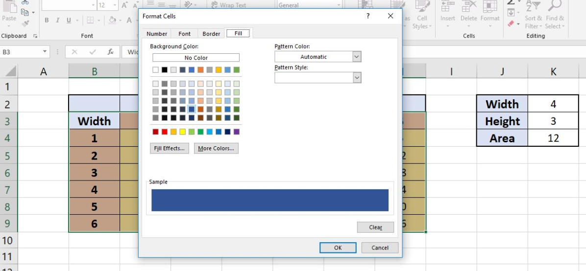 Figure 7. Defining the formatting for the cells
Step 8
Furthermore, click the “OK” button which will take you back to the Conditional Formatting Rules Manager showing the formula, format and the range of cells to which it has been applied. Click the “OK” button to close this window.
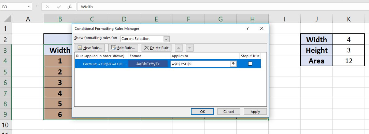 Figure 8. Conditional Formatting rules defined
Step 9
Next, the cells that approximate match lookup and formatted accordingly.
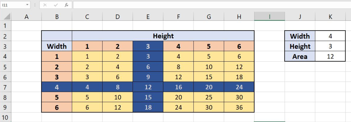 Figure 9. Result-1 of highlighted approximate match lookup according to conditional formatting criteria
Step 10
Finally, it can be seen that changing the Width and Height in the box on the right affects the formatting region.
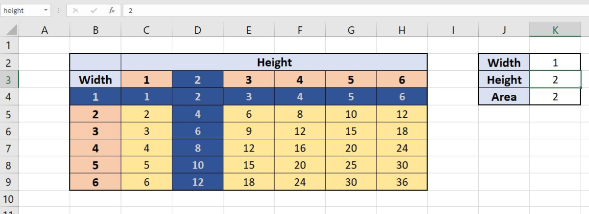 Figure 10. Result-2 of highlighted approximate match lookup according to conditional formatting criteria
Still need some help with Excel formatting or have other questions about Excel? Connect with a live Excel expert here for some 1 on 1 help. Your first session is always free.


Leave a Comment