

Conditional Formatting is a feature in Excel that allows us to change the format of cells based on a set of rules or conditions. For any given data, the format of a cell can be changed based on its content, or the contents of another cell. This step by step tutorial will help all levels of Excel users conditional format our spreadsheets.
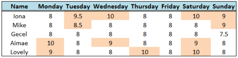
Figure 1. Final result: Conditional formatting based on the contents of a cell
Setting up the Data
Here we have a table showing the daily hours worked in a week by five employees.
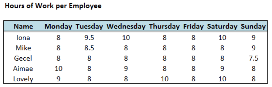 Figure 2. Sample data for conditional formatting based on the contents of a cell
To show how to use Conditional Formatting based on the contents of a cell, we want to :
- Highlight cells based on its content
Criterion: Highlight all cells with hours of work greater than 8 hours - Highlight cells based on the contents of other cells
Criterion: Highlight the names of employees who worked more than 8 hours on Sunday
Highlight cells based on its content
We want to highlight all cells with a value greater than “8” hours. Follow these steps:
- Step 1. Select the cells to be formatted. In this case, select cells C4:I8.
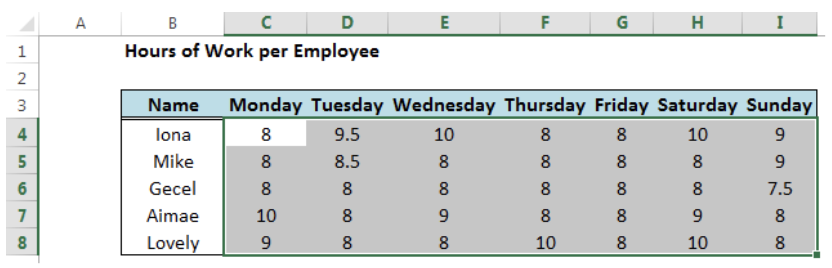 Figure 3. Selection of the data range for conditional formatting
- Step 2. Click the Home tab, then the Conditional Formatting Menu and select “New Rule”. The New Formatting Rule dialog box will pop up.
 Figure 4. Creation of a new rule in conditional formatting
- Step 3. Select the Rule Type “Use a formula to determine which cells to format” and enter this formula in the dialog box :
=C4>8
This formula evaluates the cell on whether or not it contains a value greater than 8.
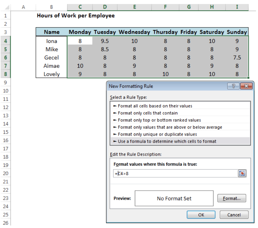 Figure 5. Entering the formula as a condition or formatting rule
- Step 4. Click “Format” and then decide on what will be the new format to apply to the cells. We can change the font, borders or fill the cells with different colors.
Example:
Select “Fill” and choose Orange, Accent 6, Lighter 60% and click OK.
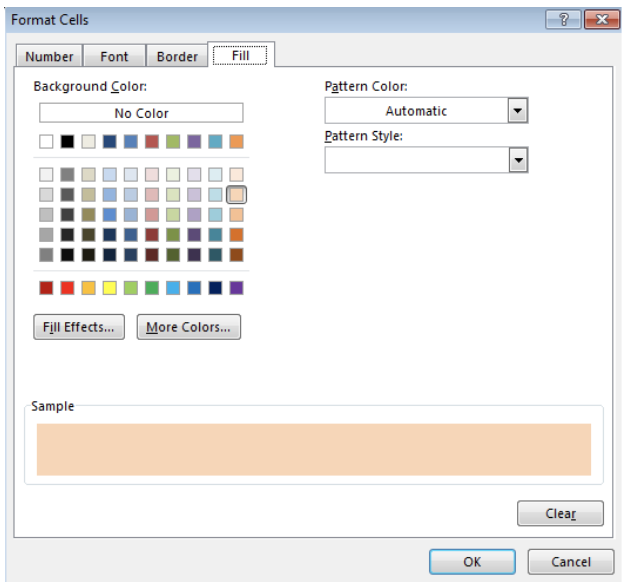 Figure 6. Selection of the format to use
 Figure 7. Completion of the new formatting rule with formula and selected format
This rule highlights all cells whose value is greater than 8.
 Figure 8. Output: New conditional formatting rule reflected in the cells containing a value greater than 8
As shown, we are able to use conditional formatting based on the contents of a cell.
Now we will try to use conditional formatting to highlight a cell based on the contents of another cell.
Highlight cells based on the contents of other cells
The uses of Conditional Formatting include changing the format of a certain cell based on another cell. It all depends on the condition that we set and the formatting rule that we create.
Example:
Highlight the names of employees who worked more than 8 hours on Sunday.
- Step 1. Select the cells to be formatted, which contain the names of employees. In this case, select cells B4:B8.
 Figure 9. Selection of the data range for conditional formatting
- Step 2. Click the Home tab, then the Conditional Formatting Menu and select “New Rule”. The New Formatting Rule dialog box will pop up.
- Step 3. Select the Rule Type “Use a formula to determine which cells to format” and enter this formula in the dialog box :
=I4>8
This formula evaluates if cells in column I “Sunday” contain a value greater than 8.
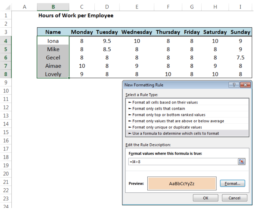 Figure 10. Entering the formula as a condition or formatting rule
- Step 4. Change the format as preferred.
Example:
Select “Fill” and choose Orange, Accent 6, Lighter 60% and click OK.
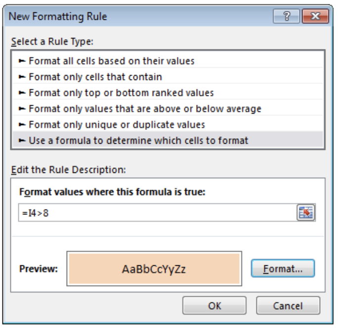 Figure 11. Completion of the new formatting rule with formula and selected format
This rule highlights the names of employees who worked more than 8 hours on Sunday, which in this case, are Iona and Mike.
 Figure 12. Output: New conditional formatting rule reflected in the names of employees with more than 8 hours work on Sunday
Most of the time, the problem you will need to solve will be more complex than a simple application of a formula or function. If you want to save hours of research and frustration, try our live Excelchat service! Our Excel Experts are available 24/7 to answer any Excel question you may have. We guarantee a connection within 30 seconds and a customized solution within 20 minutes.


Leave a Comment