

Conditional Formatting is a feature in Excel that allows us to change the format of cells based on a set of rules or conditions. There are instances when we need to highlight a row or a column, depending on the data we have and the desired results. This step by step tutorial will assist all levels of Excel users in highlighting rows or columns based on a condition.
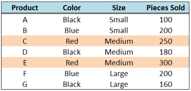
Figure 1. Using conditional formatting to highlight a row
Setting up the Data
Here we have a table showing Products A to G, with corresponding Color, Size and Pieces Sold. We want to highlight the rows for products with the color “Black”.
 Figure 2. Sample Data for conditional formatting to highlight a row
Using Conditional Formatting to Highlight a Row
To highlight an entire row, we use Conditional Formatting and enter a formula based on the required or given criteria.
- Step 1. Select the cells to be formatted. In this case, select cells B4:E10.
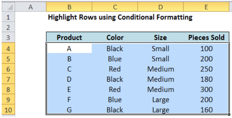 Figure 3. Selection of the data range for conditional formatting
- Step 2. Click the Home tab, then the Conditional Formatting Menu and select “New Rule”. The New Formatting Rule dialog box will pop up.
 Figure 4. Creation of a new rule in conditional formatting
- Step 3. Select the Rule Type “Use a formula to determine which cells to format” and enter this formula in the dialog box :
=$C4=“Black”
Important note:
To highlight a row, we fix the column that serves as the reference for the conditional formatting
Note that the column is fixed by using the symbol “$”. This formula triggers the conditional formatting, and the “$” before “C” ensures that the reference column is only the column for “Color”. For every row of data, the format will be changed if the “Color” is “Black”.
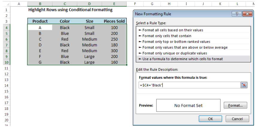 Figure 5. Entering the formula as a condition or formatting rule
- Step 4. To change the format, click “Format” and then decide on the new format to apply to the entire row. We can change the font, borders or fill the cells with different colors.
Example :
Select “Fill” and choose Orange, Accent 6, Lighter 60% and click OK.
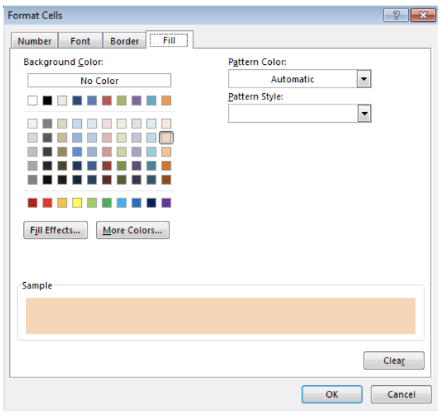 Figure 6. Selection of the format to use
 Figure 7. Completion of the new formatting rule with formula and selected format
This rule highlights the rows of data that satisfy the condition of Color=“Black”.
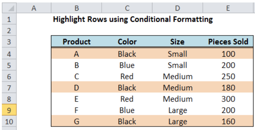 Figure 8. Output: New conditional formatting rule reflected in the rows of data with the color “Black”
As shown, we are able to change the format of the entire row for Products A, D and G with color “Black”.
There are also cases where we need to highlight a column because the data we have requires it that way.
Setting up the Data for Highlighting a Column
Here we have a similar table as the above example, only that the headers are in the leftmost side and the information per product is shown per column. In the same manner as the previous example, we want to highlight the columns for products with color “Black”.
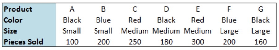 Figure 9. Sample Data for Conditional Formatting to Highlight a Column
Using Conditional Formatting to Highlight a Column
The steps for highlighting a column are similar to that of highlighting a row. The only difference is in the formula we use to satisfy the condition.
- Step 1. Select the cells to be formatted. In this case, select cells C3:I6.
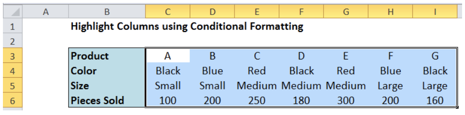 Figure 10. Selection of the data range for conditional formatting
- Step 2. Click the Home tab, then the Conditional Formatting Menu and select “New Rule”. The New Formatting Rule dialog box will pop up.
- Step 3. Select the Rule Type “Use a formula to determine which cells to format” and enter this formula in the dialog box :
=C$4=“Black”
Important note:
To highlight a column, we fix the row that serves as the reference for the conditional formatting
Note that the row is fixed by using the symbol “$” before row “4”. This ensures that the reference row is only the row for “Color”. For every column of data, the format will be changed if the “Color” is “Black”.
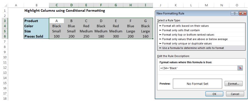 Figure 11. Entering the formula as a condition or formatting rule
- Step 4. Change the format as per your preference.
Example :
Select “Fill” and choose Orange, Accent 6, Lighter 60% and click OK.
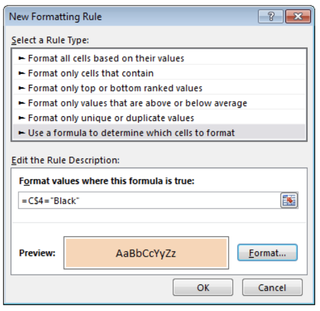 Figure 12. Completion of the new formatting rule with formula and selected format
This rule highlights the columns of data that satisfy the condition of Color=“Black”.
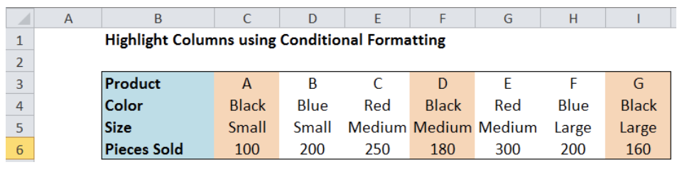 Figure 13. Output: New conditional formatting rule reflected in the columns of data with the color “Black”
We have successfully highlighted the columns for Products A, D and G with color “Black”.
Other examples
Criteria: Highlight rows or columns for products with greater than 200 pieces sold.
Follow Steps 1 to 4 as discussed above, but use the formula: Pieces sold>200
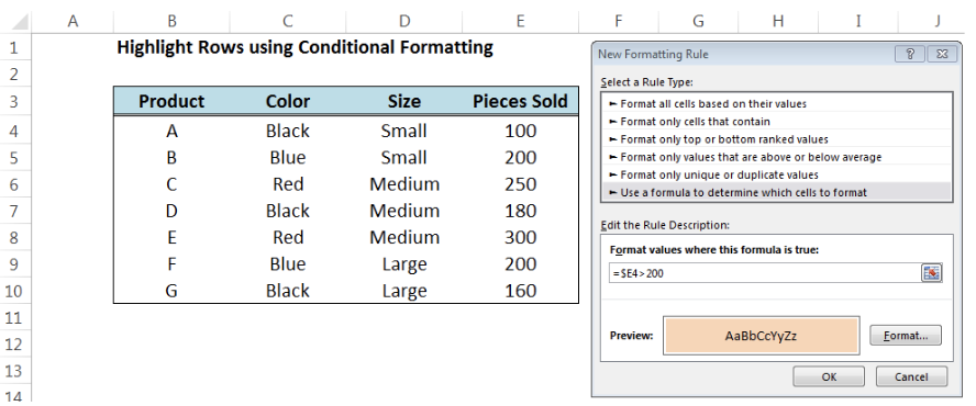 Figure 14. Entering the formula =$E4>200 and setting the format
 Figure 15. Output: New conditional formatting reflected for products with >200 pieces sold
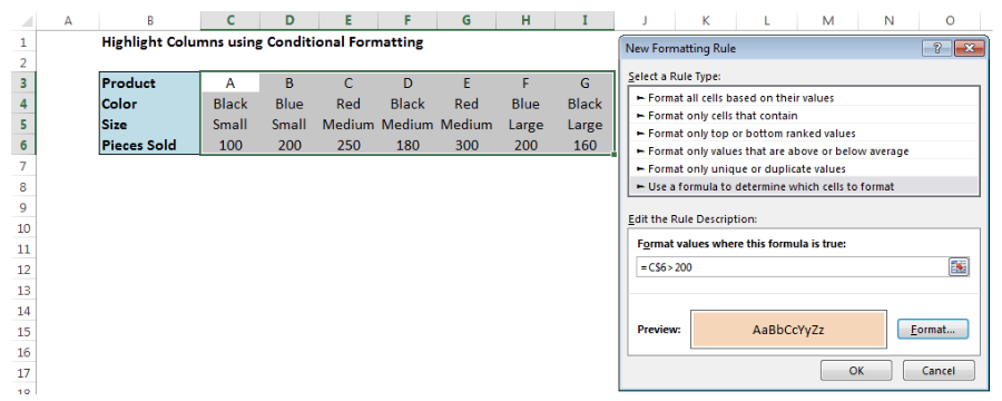 Figure 16. Entering the formula =C$6>200 and setting the format
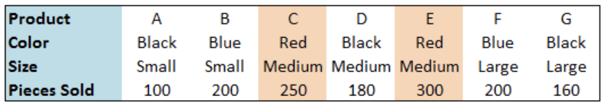 Figure 17. Output: New conditional formatting reflected for products with >200 pieces sold
Most of the time, the problem you will need to solve will be more complex than a simple application of a formula or function. If you want to save hours of research and frustration, try our live Excelchat service! Our Excel Experts are available 24/7 to answer any Excel question you may have. We guarantee a connection within 30 seconds and a customized solution within 20 minutes.


Leave a Comment