How to use color code in Excel – Excelchat

We can use conditional formatting to automatically change the cell background color based on the data value in the cell.

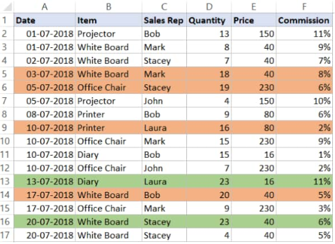Figure 1. of Cell Color in Excel

Whenever we are dealing with large amounts of data in Excel, we can decide to pick out matching values and highlight them by using a specified color of font or cell background

How to Color Code in Excel

If we desire to change Excel color code based on the values in the cells, we must apply conditional formatting.

Since, we sometimes want to highlight an entire column (or row) instead of just a cell or two; this is why we will base the color code in Excel on matching values within the cells.

Let’s say we have the sales roaster containing the details of purchases made at a store during the year;

1. We begin by collecting the data available to us in well labelled columns of our Excel worksheet:

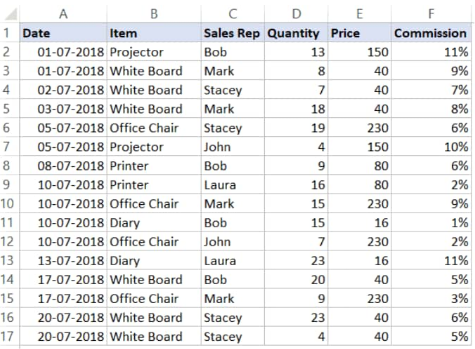Figure 2. of Cell color in Excel

Our goal here is to highlight all the sales records for the Sales Rep named Bob.

2. Select the whole dataset on our worksheet (A2:F17) and then click on the “Home” tab on the top left side of our worksheet:

Figure 3. of Home Tab in Excel

3. In the “Styles” group, open “Conditional Formatting”:

Figure 4. of Conditional Formatting Tab in Excel

4. Open ‘New Rule’:

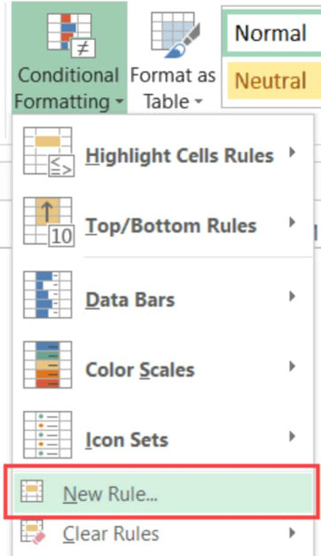Figure 5. of New Conditional Formatting Rule in Excel

5. A ‘New Formatting Rule’ fly out appears, click on the ‘Use formulas to determine which cells to format’ button:

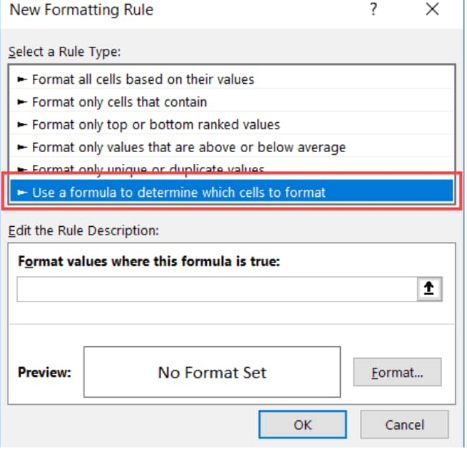Figure 6. of New Formatting Rule in Excel

6. In the formula dialogue box, input the following operation:

=$C2=”Bob”

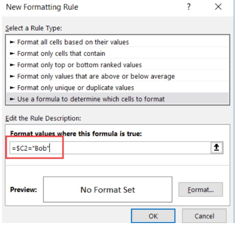Figure 7. of New Formatting Rule in Excel

7. Click on the ‘Format’ icon.

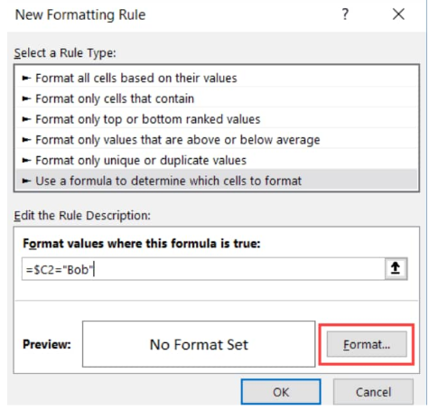Figure 8. of New Formatting Rule in Excel

8. In the next dialog box that emerges, we will set the Excel color which we want to use in highlighting the specified rows.

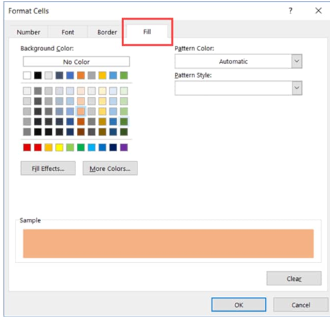Figure 9. of Format Cell Color in Excel

9. Clicking “OK” will highlight every row where Sales Rep “Bob” is located with the specified Excel color:

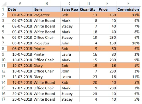Figure 10. of Color Formatting in Excel

Conditional Formatting in Excel checks the data in every cell of our worksheet for the given condition, =$C2=”Bob”

So when it is analyzing the cells in row A2, Excel checks out the cell C2 for the name “Bob”. If it does, the cell becomes highlighted, otherwise it doesn’t.

Note

Be sure to use the dollar sign ($) in Excel before the column’s alphabet – $C1 – this will lock the column to remain as “C”; this way, when cell A2 gets checked by the formula, it also checks C2; similarly, when A3 gets checked for our criteria, it will also check C3.

This helps to ensure the entire row is highlighted by conditional formatting.