Learn How to Work With Images in Excel

When you think of Excel, you might only picture a spreadsheet full of data. But, the program has the ability to represent information in a variety of ways. One thing you can do is add images to Excel to make the data more meaningful.

This guide explains the various ways that you can work with images in Excel, such as inserting an image, manipulating images, and creating watermarks. As always, Excelchat is available 24/7 to provide one-on-one assistance for learning and troubleshooting.

Learn how to work with Images in Excel.

Insert an Image in Excel

All versions of Excel give you the ability to insert images that are stored on your computer. If you have Excel 2013 or Excel 2016, you can also insert images from web pages and online storage locations such as Facebook, Flickr, and OneDrive.

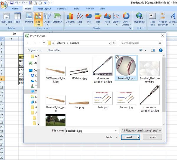
To insert an image from your computer, start at the cell where you want the image to go and then go to the Insert tab and choose Pictures.

Excel screen shot of Insert pictures box.

When the dialogue pop-up box appears, navigate to the image you want to insert into your spreadsheet and click Insert. If you want to insert several images at once, just hold down the CTRL key as you select images before hitting Insert.

Excel screen shot of insert clip art box.

Modify an Image in Excel

Once you’ve inserted an image in Excel, you might want to make some changes to it. Excel gives you the tools to format images in a variety of ways. You can add shading, framing, colored borders, picture effects, bring the image to the front of the text or put it in the background, resize, and rotate your image.

The tools to do this are located under Picture Tools > Format. If you simply click on your picture in Excel, your upper ribbon will default to this menu.

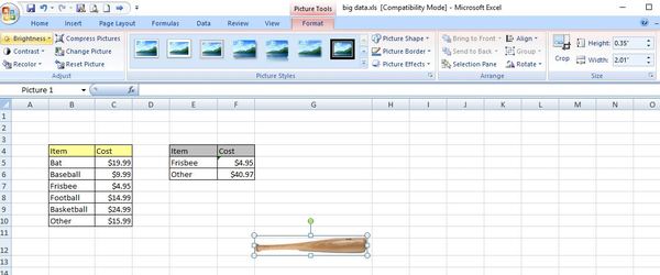
Format picture menu screen shot in excel.

You can also manually resize an image by clicking on it and dragging any of its edges. In the case of the baseball bat (above), this can be resized in this fashion. If you want to keep the same aspect ratio, only drag on one of the four corners for resizing.

To place an image firmly in a cell, just hold down the ALT key, and then use your mouse to move that image into the cell. It will then arrange itself and “snap” into that cell as it gets close to it. However, if you hide, resize, or delete that cell, row, or column, later, this could affect this image. You would also have to lock the image to the cell to protect it.

Lock an Image in Excel

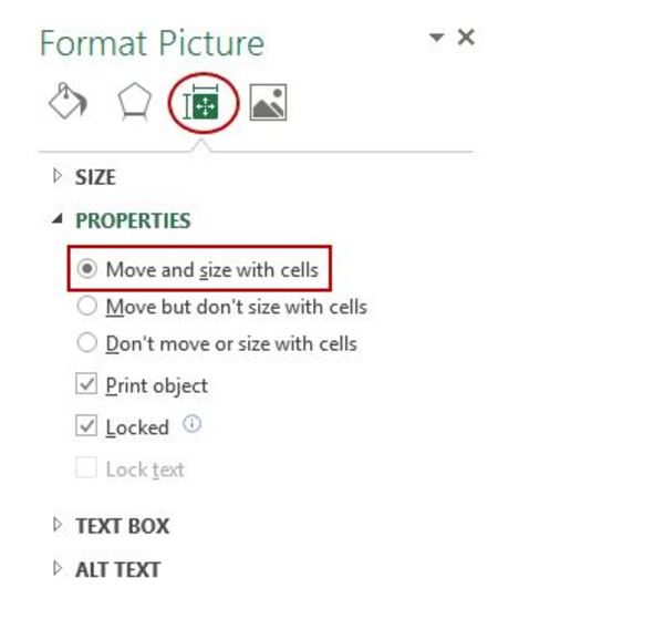
Locking an image to cell ensures that it will filter, hide, and move along with that cell. The steps to lock an image to a cell are simple.

Choose the image that you want to lock and then right-click. Select Format Picture. When the dialogue box appears, choose the Size & Properties options and, under Properties, choose “Move and size with cells.” Now your image is locked to the cell.

Format picture box in excel.

Insert an Image Into a Comment

Excel comment boxes are small boxes that appear when your mouse hovers over the top right corner of a cell, where a “comment” has been left. These provide additional information about the information in the cell, and they can also hold images.

First, you’ll need to insert a comment box for a cell. You do this by right-clicking on the cell and choosing Insert Comment. (Shift + F2 also accomplishes this). You may want to delete any optional text that shows up in your box since this will interfere with your image.

Click on the comment box itself (not the inside of it) and then right-click and choose Format Comment. This will bring up a dialogue box. Choose the Colors and Lines tab. Click on the Fill Color drop-down box and choose Fill Effects at the bottom. Select the Picture tab and find your image. Click OK.

Select picture popup box in excel.

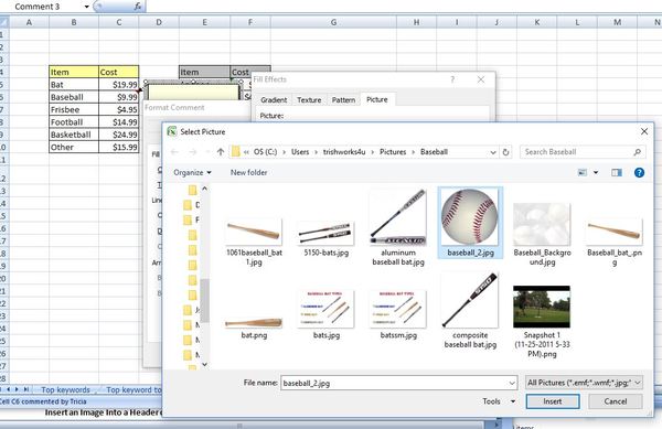
Now you have an image in your comment box.

Excel spreadsheet screen shot of an image next to data.

Insert an Image Into a Header or Footer

Excel also allows you to insert an image into the header or footer, which you can use as a watermark. To do this, go to Insert > Text > Header & Footer. Choose either the header or footer portion of your spreadsheet to insert the image (you can switch between the two from buttons at the top of the page).

You have three places in a header or footer to put an image, in the left, right, or center box. Put your cursor where you want the image to appear.

The Design tab will be active, and you can choose Picture from the options on the ribbon. A picture dialogue box will open. Navigate to the image you want to be included in the header or footer and click Insert.

Insert picture box in excel.

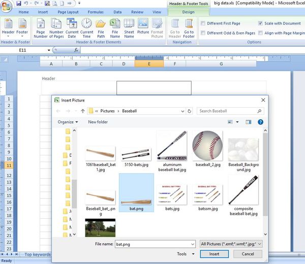
After you do this, you won’t actually see the image in your header or footer but rather the code &[Picture]. If you click on any cell in your worksheet, you’ll then be able to see the watermark.

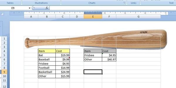
Excel sheet with data and image of a large baseball bat.

Note: When you insert a watermark, Excel will remain in Page Layout View. If you switch to Normal view, the watermark will still be there and will print with the worksheet, but you won’t see it on your screen.

Need Some More Help With Images in Excel?

While these explanations cover some of the most common things that you’ll do with images in Excel, you might still run into some roadblocks or have a unique issue. Maybe you’d just rather have some one-on-one help to save time.

Excelchat provides fast and friendly live chat help for any issues related to Excel. Learn how to use the program or solve a problem that is keeping you from moving forward with your work — in just a few minutes. Your first session is always free.