

Conditional formatting is used to highlight the cells where a given condition is met. However, if we want to highlight the cells that meet multiple conditions, then conditional formatting with AND function is used.
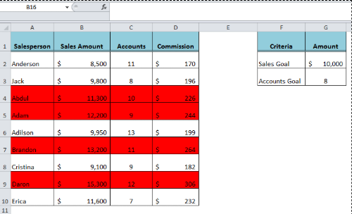
Figure 1. Final result
AND Function
The AND function is used to evaluate multiple conditions and it returns TRUE when all the conditions are met, otherwise returns FALSE. Therefore, the custom rule of conditional formatting with AND function triggers to highlight selected cells or rows when all the provided conditions are met. We have a dataset of salespersons accounts and their sales amounts. We want to evaluate the following conditions to highlight the rows where salespersons exceed both sales and account goals
- Sales Amounts in column B are greater than or equal (>=) to the Sales Goal of $10,000
- AND Accounts in column C are greater than or equal (>=) to the Accounts Goal of 8
Using conditional formatting with AND function the custom formula rule is created to evaluate both given conditions in the following formula syntax:
=AND(Sales Amount >=Sales Goal, Accounts >=Accounts Goal)
OR
=AND($B2>=$G$2,$C2>=$G$3)
 Figure 2. Salespersons’ dataset with conditions to evaluate
Applying Conditional Formatting
We use conditional formatting with AND function to highlight rows where above two conditions are met. To add conditional formatting in this case, follow the following steps:
- Select the range of cells where salespersons data is entered, such as A2: D10
- On the Home tab, click Conditional Formatting and then click New Rule
- Click the option “Use a Formula to Determine Which Cells to Format”
- In the formula box, enter
=AND($B2>=$G$2,$C2>=$G$3) - Click the Format button and select the Formatting option, such as Fill > Red color > OK
- Click OK
 Figure 3. Applying Conditional Formatting with AND function
Figure 4. Highlighting rows that meet both conditions
Instant Connection to an Expert through our Excelchat Service:
Most of the time, the problem you will need to solve will be more complex than a simple application of a formula or function. If you want to save hours of research and frustration, try our live Excelchat service! Our Excel Experts are available 24/7 to answer any Excel question you may have. We guarantee a connection within 30 seconds and a customized solution within 20 minutes.


Hello