

We can have alternate colors by shading alternate rows or shade alternate columns in the worksheet (also called color banding) to make it easy for readers to scan through. To shade alternate rows, or column, we can adopt a preformatted table by clicking on Tables and select the desired table style.
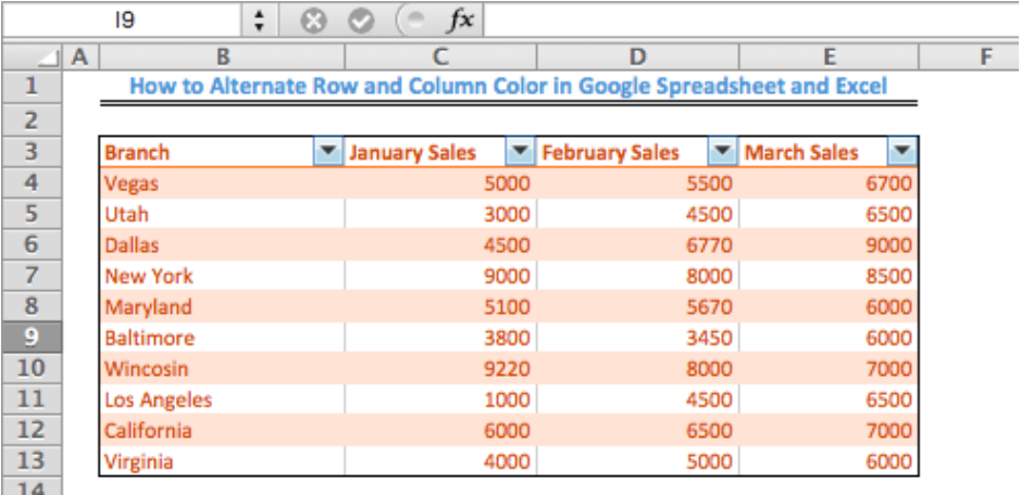 Figure 1 – Result of How to Alternate Colors
How to Make Rows Alternate Colors
The steps below demonstrate how we can alternate row colors:
- We will select the range of cells (B3:E13) where we want alternating row colors
- We will click on Insert to convert our range to a table
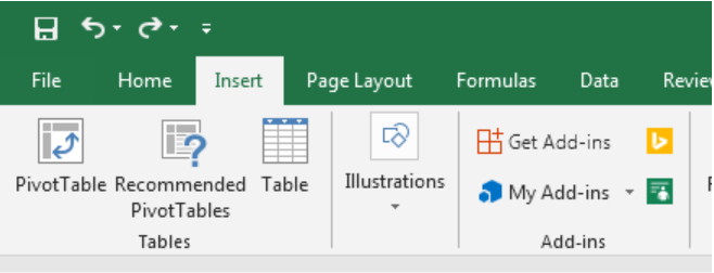 Figure 2 – Click on Insert
- We will click Table Styles to select one that has alternate shading across rows.
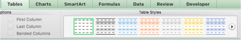 Figure 3 – Choose a Table Style to Alternate color rows
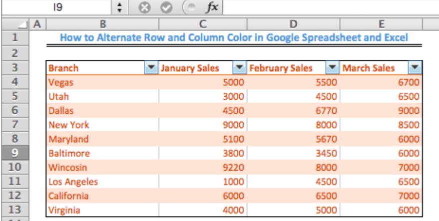 Figure 4 – Result of alternating colors across rows
How to Make Columns Alternate Colors
To change the shading from rows to columns, we will select the table range B3:E13. Under the Tables tab, we will uncheck the Banded Rows box and check the Banded Columns box.
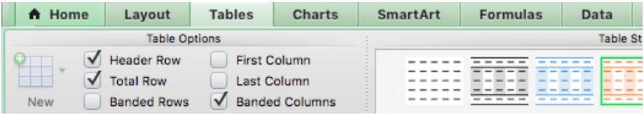 Figure 5 – Change the Color Shading from Rows to Columns
Note: Rows or columns are automatically colored as we keep adding rows or columns to our data.
Using Conditional Formatting to Apply Banded Rows and Columns
We can also use conditional formatting to shade alternate rows.
- We begin by selecting the range of cells where we want alternate row shading
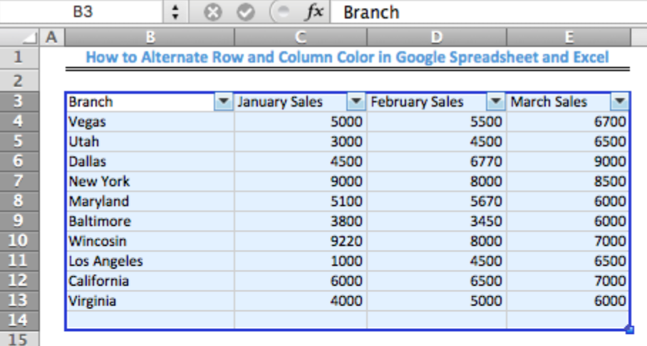 Figure 6 – Selecting the Range for alternate row colors
- On the Home tab, in the Styles group, we will select Conditional Formatting.
 Figure 7: Select Conditional Formatting
- We will Select New Rule.
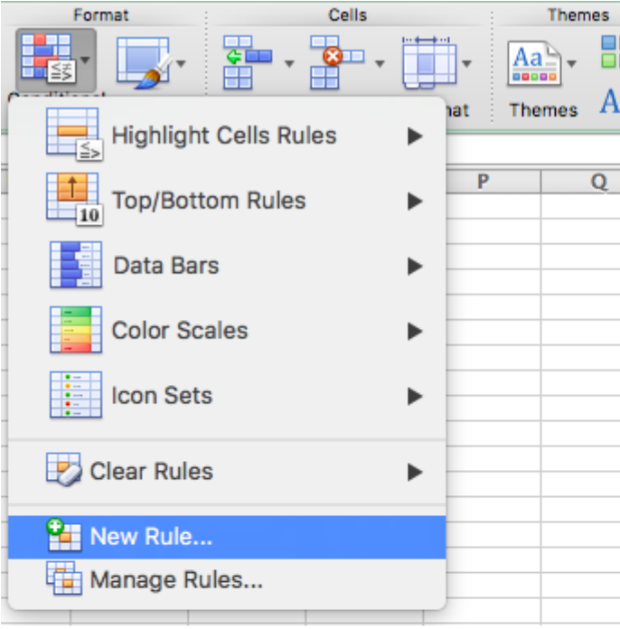 Figure 8: Select New Rule under the Conditional Formatting dropdown
- Make sure the Style section is “Classic”. It is sometimes set to 2-Color Scale by default. Change it to Classic, then on the next dropdown, select ‘Use a formula to determine which cells to format’.
- Enter the formula
=MOD(ROW(),2)
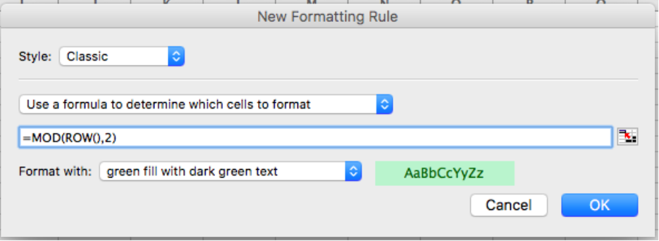 Figure 9: Enter the Formula to make the rows alternate colors
- We will select a formatting style and click OK.
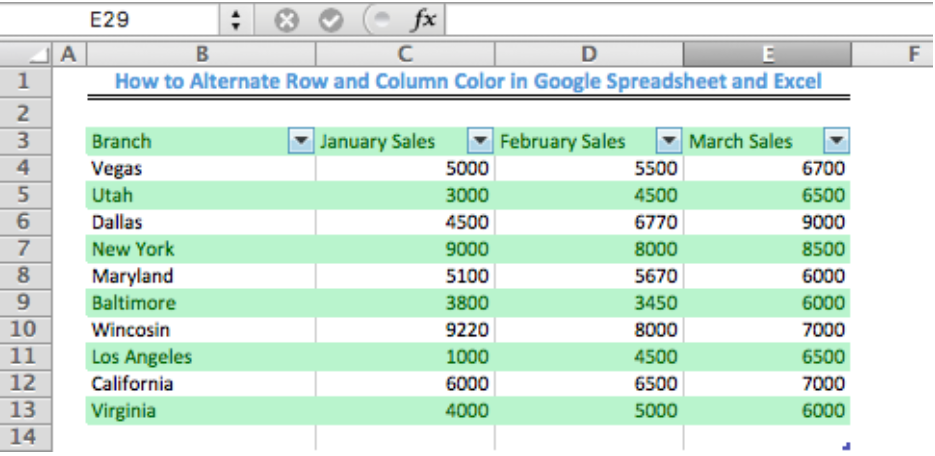 Figure 10: The Table after alternate row shading is done across the rows
- To shade the columns alternately, we will follow all the steps above except that the formula would, in this case, be =MOD(COLUMN(),2). The table would then look like this:
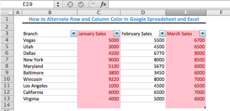 Figure 11: Alternating Colors in columns
Note: The modulo or MOD(m,n) function gives the remainder when m is divided by n. So, the formula instructs Excel to alternate row colors for all odd colored rows with the specified color.
Instant Connection to an Excel Expert
Most of the time, the problem you will need to solve will be more complex than a simple application of a formula or function. If you want to save hours of research and frustration, try our live Excelchat service! Our Excel Experts are available 24/7 to answer any Excel question you may have. We guarantee a connection within 30 seconds and a customized solution within 20 minutes.


Leave a Comment